Xenoplasy

A major obstacle in studying morphological evolution is homoplasy. This occurs when the same (or similar) traits are evolved independently in different lineages (convergences), and are positively selected for or incompletely sorted within a lineage (parallelisms, homoiologies). Traits that not sort following the true tree create incompatible signal patterns, and, eventually, topological ambiguity. No matter which inference method we use, we end up with several alternative trees that combine aspects of the true tree with artificial branching patterns.

Homoplasy is the rule, while trait sorting is the exception. Consequently, we have to expect that any morphology-based tree will have more wrong branches than correct ones.

For extant group of organisms, a simple solution to the problem is to analyse morphological traits in the framework of a molecular phylogeny. The genetic data provides us with an independent, best-possible tree. By mapping the morphological traits on this tree, we can evaluate their potency as phylogenetic markers.

But what if our group of organisms is not the product of a simple repeated dichotomous splitting pattern? What if there were anastomoses as well? That is, the morphological traits are not the product of mere (incomplete) lineage or incomplete gene sorting (the latter is called "hemiplasy") but fusion of traits in different lineages. Thus, a tree is not enough to explain the genetic data? What does this imply for the morphological differentiation we observe?

Take the London Plane (Platanus x acerifolia or P. x hispanica), for example, which is a tree that many of us are familiar with. In case you don't know the name: they are the large trees with a patterned bark and deeply lobed leaves and fluffy fruiting bodies found in abundance in parks and alleys throughout the world. It's a cultivation-hybrid (17th—18th century) of the North American plane tree, Platanus occidentalis, and its distant eastern Mediterranean relative, P. orientalis. These are genetically and morphologically distinct species. Their history is summarized in the following doodle (Grimm & Denk 2010).

Each line represents a semi-sorted nuclear gene region. The split between proto-PNA-E (SW. U.S., NW. Mexico, E. Mediterranean) and proto-ANA (Atlantic-facing Central America, E. U.S.) must have been > 12 myrs ago (last Platanus of Iceland). The minimum air distance between the sister species P. orientalis and P. racemosa is ~11,500 km (via the Arctic). Interestingly, fossils from that time and later (including western Eurasia) have more ANA-clade morphologies: P. orientalis- and P. racemosa-types pop up ~5 Ma. Both ANA and PNA-E clade have distinct morphologies. With respect to the individual gene trees, those exclusively shared by P. palmeri and P. rzedowski with P. occidentalis s.str. and P. mexicana of the ANA clade could be adressed as "hemiplasies".

If you look at the leaves and fruits of London Planes, you can find everything in between the two endpoints; and the same holds for their genetics. The London Plane is much hardier than Europe's own P. orientalis and more drought-resistant than its hardier North American parent. With climate change going on, the hybrid will eventually meld with the European species entirely. And, thanks to what we call "hybrid vigor", given a few millions of years, it might consume its other parent, too. London Planes have been re-introduced into the Americas; and P. orientalis has become an invasive species in California, where it has started to hybridize with its local sister species P. racemosa. Now imagine a future researcher of Platanus evolution having to deal with a highly complex accumulation of Platanus fossils in the Northern Hemisphere, while being able to study only the left-over complex genetics of a single species that replaced two.

This is where a recently coined new concept comes in: xenoplasy.

Yaxuan Wang, Zhen Cao, Huw A. Ogilvie, Luay Nakhleh (2020). Phylogenomic assessment of the role ofhybridization and introgression in trait evolution. bioRxiv doi: 10.1101/2020.09.16.300343

Xenoplasies are traits that originate from hybridization and subsequent introgression. In standard phylogenetics, they would act like any homoplasious character, but their distinction is that they are not independently involved. They are captured via lineage crossing, and reflect a common ancestry.

Example for a trait incongruent with the species tree, representing a xenoplasy obtained by introgression of I1-A lineage which evolved the trait into I3-B lineage, part of the I2 clade. Pending how far they are affected by incomplete lineage sorting (ILS) and introgression, individual gene may result in any of the three possible genealogies. Modified after Wang et al. (2020), fig. 1.

As such, their phylogenetic weight (information content) equals that of the anyhow rare classic autapomorphies or synapomorphies (fide Hennig), and this weight is higher than that of the more common homoiologies, shared apomorphies or symplesiomorphies. Note, in the palaeozoological cladistic literature, sorted versions of the latter three are often called synapomorphies – any lineage-specific, derived trait ("synapomorphy") may be lost / modified in some sublineage(s), or rarely pop-up outside the lineage.

Wang et al. provide an analytical framework for identifying a trait as xenoplasy, and assessing the probability for it ("xenoplasy risk factor"). If you're interested in the mechanics, check out the pre-print. The mathematical part of my brain has been dormant for most of the last two decades (when I exchanged chemistry for geology-biology), so I'm more into possible applications to explore this new concept.

Where to look next

The Wang et al. real-world example (Jaltomata) is, however, not very appealing. The problem is that, to look for xenoplasy, we need data that requires us to infer an explicit phylogenetic network (in the strict sense) to start with. In addition, we could use a morphological partition: scored morphological traits; which is usually absent. Last, identifying xenoplasies would make most sense for traits that can be traced in the fossil record, not only to identify potential products of past reticulation but have a better grip on placing critical fossils. Often overlooked by neontologists, fossils are the only physical proof that a lineage was at a certain place at a certain point in time. So, here's two examples: beeches and bears.

Beeches are a small genus of extra-tropical angiosperm trees with a pretty well understood fossil record. Morphologically, their differentiation is very hard to put into a tree, as shown here.

A morpholgy-based Neigbor-net of fossil (open circles) and extant beech (closed circles) taxa. Coloration gives the (paleo-)geographic distribution (abbreviated as three letters). For more background and information see my Res.I.P. post: The challenging and puzzling ordinary beech – a (hi)story

Mapping species-discriminating traits on a tree would be of little help here, because the modern species are the product of recurrent phases of mixing and incomplete sorting. I have summarized  this in the following doodle, depicting the diversification and propagation of 5S-IGS variants (a non-transcribed, poly-copy, multi-array intergenic nuclear spacer) in a still very small sample.

A doodle summarizing differentiation patterns in a sample of 686 "representative" 5S-IGS variants obtained using high-throughput sequencing of six beech populations of western Eurasia and Japan (Simone Cardoni et al., to be submitted in the near future; see Piredda et al. 2020 for a similar analytical set-up).

The people involved in researching this project (drawn by passion rather than resources) don't have the resources to generate the NGS data needed to construct a species network for all of the species of beech, like Wang et al.'s Jaltomata data. But given that there are only 9–10 species, it would be easy prey for a well-funded research group. If you are interested, but don't know how to get the material and are unfamiliar with beeches, feel free to contact the senior author of Piredda et al. 2020, Marco Simeone — new beech-enthusiasts are always welcomed by this group.

Bears are one of the best-studied extant mammal predators, and they also have a decent fossil record. This is probably the reason that Heath et al. (2014) used bears as the case study when introducing their new molecular dating approach: the fossilized-birth-death dating.

A fossilized birth-death dated tree of bears (modified from Heath et al. 2014, fig. 4). The numbers in brackets give the number of fossil taxa (extinct genera, Ursus spp.) listed on Wikipedia.

As nice as it looks (and done), their analysis is pretty flawed from an evolutionary point of view. Their dated tree only reflects a single aspect of bear evolution and may involve branch-length artifacts. Heath et al. relied on complete mitochondrial genomes, which they combined with a single nuclear protein-coding gene. Mitochondrial genes reflect only the maternal lineage; they did not date a species tree but a mitochondrial genealogy. Paternal and biparentally inherited gene markers (which includes nuclear genes) tell very different stories about species relationships (this is why we also used the bears as example data for Schliep et al. 2017).

Strict, branch-length ignorant Consensus network of three trees inferred using species-consensus sequences generated from three sets of data: biparentally inherited nuclear-encoded autosomal introns (ncAI), paternally inherited Y-chromosomes (YCh) and maternally inherited mitochondrial genes (complete set; mtG). This is clearly not the product of a strictly dichotomous evolution. Thick lines: edges found in Heath et al.'s chronogram (= mitochondrial genealogy).

And while it may be that morphology reflects more the maternal than the paternal side, it has never been tested. Neither how morphology fits with the coalescent species tree. Which would be a network, as shown below.

Gene flow in bears within the last 5 myrs (estimate; from Kumar et al. 2017).

How Heath et al. linked the fossils to clades might have been just as wrong as it was right (note that FBD dating is much less biased by mis- or unoptimal placed fossils than traditional node dating). Hemi- and xenoplasy must be considered here. In addition to the highly incongruent paternal and maternal genealogies, we know that even the morphologically most distinct sister species (grizzlies, a special form of Brown Bear, and polar bears) can produce vital offspring ("Grolar") with morphological traits from either side of the family (usually, the Grizzly-side dominates).

Wildlife services usually kill these hybrids as they are considered to speed up the decline of polar bears (they are food competitors). However, with the (possibly inevitable) melting of the polar caps, these hybrids could be instrumental in the survival of a bit of Polar Bear legacy, in the form of genetic diversity not found in brown bears, and xenoplasies. If two highly distinct bear species hybridize today in the wild due to (in this case: human-induced) environmental pressure, their ancestors probably have done so in the past in reaction to shifting habitats and migration patterns.

Given how long bears have intrigued researchers, there are plenty of classic morphological studies involving fossils; and, in the light of the vast amount of molecular data (including ancient DNA!) that have been collected for bears, it should be pretty easy to apply Wang et al.'s new approach to bears. For example, is the Cave Bear a dead-end side lineage, intrograde or hybrid dead-end? Mitochondrial-wise Cave bears are placed as sister to Brown and Polar bears but that's just because of their provenance. Like chloroplast genealogies in plants, mitochondrial genealogies in animals typically show a strong geographic correlation. Especially in bears, the mothers and daughters don't migrate as much as the fathers and sons.

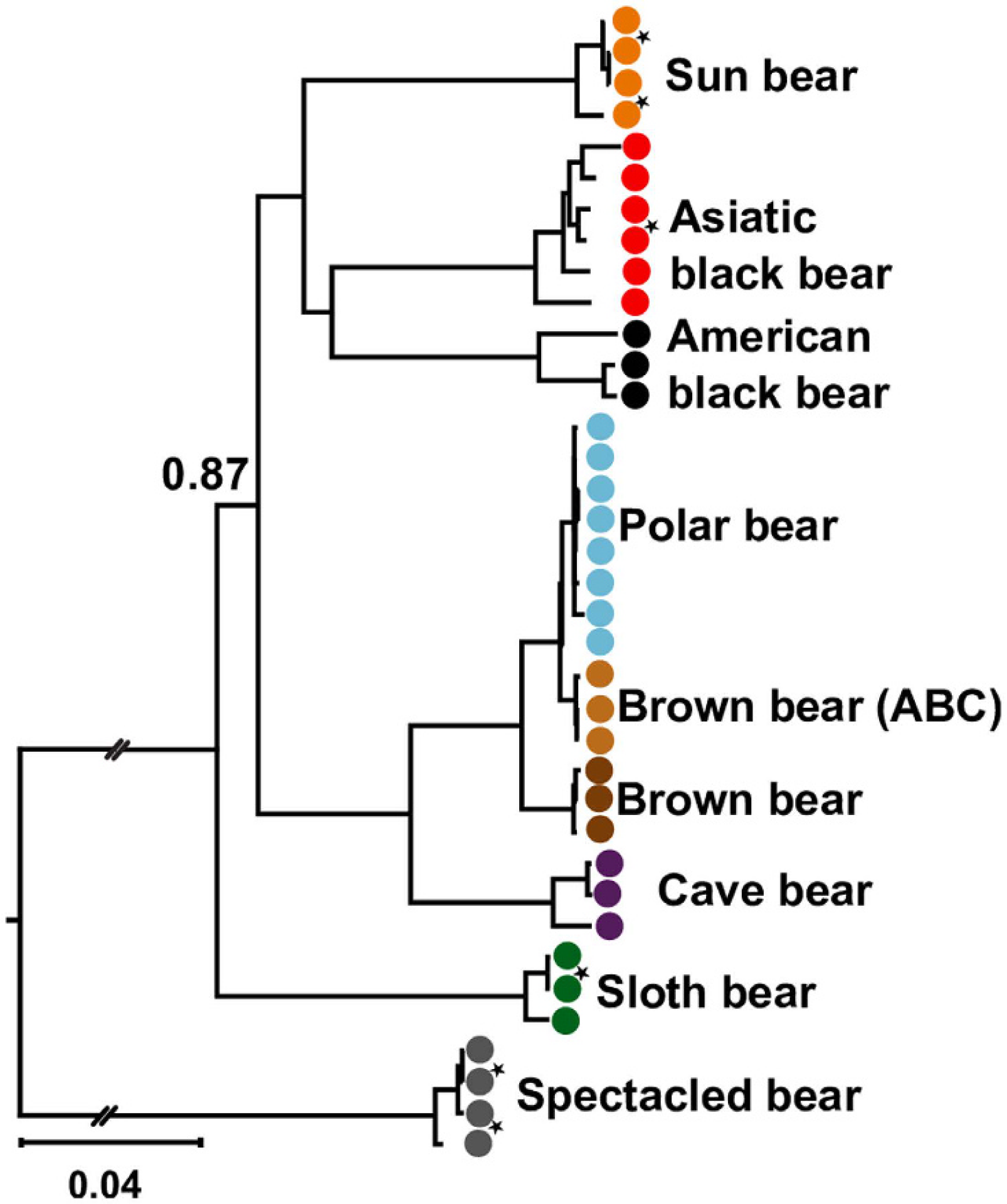
Mitochondrial genealogy of bears including Cave bears (Kumar et al. 2017, fig. 3), the famous European bears of the Ice Ages. ABC bears are insular brown bears living on the subarctic Admirality, Baranof and Chichagof islands of the Alexander archipelago known as natural example for gene flow between Brown and Polar bears (Kumar et al. 2017, fig. 1, provides a map of current distribution of bears).

Postscriptum

Birds are another animal group that likes to diversify into many species, some of which love to transgress recently established species barriers, forming hybrid swarms. These are actually dinosaurs, a group exclusively studied using cladistic analyses of morphological traits providing non-tree-like signals — mostly homoplasies, a lot of not-really-synapomorphies (good deal are probably homoiologies), and, it wouldn't surprise me, one or another xenoplasy. Or can we assume they were much to advanced to hybridize and intrograde?

Cited literature

• Grimm GW, Denk T. 2010. The reticulate origin of modern plane trees (Platanus, Platanaceae) - a nuclear marker puzzle. Taxon 59:134–147.
• Heath TA, Huelsenbeck JP, Stadler T. 2014. The fossilized birth–death process for coherent calibration of divergence-time estimates. PNAS 111:E2957–E2966.
• Kumar V, Lammers F, Bidon T, Pfenninger M, Kolter L, Nilsson MA, Janke A. 2017. The evolutionary history of bears is characterized by gene flow across species. Scientific Reports 7:46487 [e-pub].
• Piredda R, Grimm GW, Schulze E-D, Denk T, Simeone MC. 2020. High-throughput sequencing of 5S-IGS in oaks: Exploring intragenomic variation and algorithms to recognize target species in pure and mixed samples. Molecular Ecology Resources doi:10.1111/1755-0998.13264.
• Schliep K, Potts AJ, Morrison DA, Grimm GW. 2017. Intertwining phylogenetic trees and networks. Methods in Ecology and Evolution 8:1212–1220.

Rogue dinosaurs, an example from the Aetosauria

In several earlier posts (a non-comprehensive link list can be found at the end of the post), I outlined how networks, tree-sample (Consensus networks, SuperNetworks) or distance-based (Neighbor-nets) may be of practical help, especially when we study phylogenetic relationships of extinct organisms.

In this post, I will further explore this by looking at a matrix for Aetosauria (Parker 2016, PeerJ) that provides an overall (relatively) strong and unambiguous signal. [NB: The reason, I prefer to use PeerJ papers as examples is that it is one of the very few journals that is open access and has a strict open data policy — to publish there, authors have to give access to the used data.]

In the abstract of the original paper, we read the following:

Nonetheless, aetosaur phylogenetic relationships are still poorly understood, owing to an overreliance on osteoderm characters, which are often poorly constructed and suspected to be highly homoplastic. A new phylogenetic analysis of the Aetosauria, comprising 27 taxa and 83 characters, includes more than 40 new characters that focus on better sampling the cranial and endoskeletal regions, and represents the most comprehensive phylogeny of the clade to date. Parsimony analysis recovered three most parsimonious trees; the strict consensus of these trees finds an Aetosauria that is divided into two main clades: Desmatosuchia, which includes the Desmatosuchinae and the Stagonolepidinae, and Aetosaurinae, which includes the Typothoracinae.

Parker's (2016) fig. 6 shows the results of the "initial analysis" (click to enlarge, colored annotations added by me).

Systematic groups based on clades are abbreviated (see next graph for full names).

A is a "Strict component consensus" of the 30 inferred MPTs (most parsimonious trees), B the Adams consensus. C the Majority rule consensus, branch labels give percentages for branches not found in all MPTs. D a "Maximum agreement subtree after a priori pruning of one taxon (black star) within the upper clade.

Parker's (2016) fig. 7 then shows the preferred result: a "reduced strict consensus of 3 MPTs" with the red star taxon removed, and (rarely seen in dinosaur phylogeny papers) branch-support — including Bootstrap support values below 70, which are very rarely reported in the literature (from my own experience it seems that editors of systematic biology journals don't like them).

Removal of one rogue taxon (called a "wildcard" in paleozoology), Aetobarbakinoides brasiliensis, substantially reduced the number of MPTs. Nonetheless, many branches have low support, and hence also the clades (used here as synonym for monophyla) derived from them – Parker uses branch-based ("stem"-based, brackets on his tree), and node-based taxa (dots).

Low branch support may or may not matter

There are two possible reasons for low branch-support:

• non-discriminatory signal: any alternative branching pattern receives diminishing support
• internal signal conflict: two (or more) alternatives receive similar support.

Mapping the support on the preferred (inferred) optimal tree cannot tell us whether it's the one or the other — only Support consensus networks can visualize this. Since we are interested in the rogue, I re-ran the parsimony BS analysis (10,000 quick-and-dirty replicates, following Müller 2005, BMC Evol. Biol. 5:58) including Aetobarbakinoides brasiliensis.

Support consensus network based on 10,000 parsimony BS pseudoreplicates. Trivial splits collapsed, only splits are shown the occured in at least 20% of the BS replicates.

The decreased/low BS support within the most terminal (root-distant) subtrees, the Des'ini and Par'ini, relates to conflicting alternatives involving one or two OTUs. In the case of Des'ini, it is the affinity of Lucasuchus and NCSM 21723, while in the case of Par'ini an alternative (recognizing Tecovasuchus as sister to the remainder) is found in 1 out of three BS pseudoreplicate trees. The diminishing support for basal relationships (root-proximal branches/edges) is due to the general lack of discriminatory signal (BS any alternative < 25). However, there are very few situations in which the best-supported alternative differs much from that in the preferred tree. For instance, any alternative to a Stag'inae sister relationship has even less than BS = 24 (BS = 27 in Parker's "reduced" tree).

Our rogue, however, is not really a 'wildcard'. The scored characters simply put it much closer to the outgroup than is any other ingroup taxon. A simple explanation could be that it is a most primitive (least derived) member of the Aetosauria. Another possibility is that it lacks any critical trait needed to place it within the ingroup. Since the deep splits within the Aetosauria rely on very few character changes, we can put it in different position down here and the tree will still have the same number of inferred changes.

Trivial and non-trivial taxa

The cladograms typically shown provide limited information about the signal in the underlying matrix, its strength and weaknesses, even when not "naked" but annotated using branch-support values. Given that there are no severe overlap gaps in the data, a very quick alternative is the Neighbor-net (a necessary addition, in my opinion).

Bold edges correspond to branches (hence: clades) in Parker's preferred tree.

Using this, we can directly depict which groups, potential clades, draw substantial (partly trivial) character support.

For instance, according to Parker's tree and following cladistic classification, Stagonolepis is an invalid taxon: one species (St. robertsoni) is part of the Stag'inae clade, the other (St. olenki) is of the Des'inae clade. Character support is, however, nearly non-existent (Bremer value = 1 and BS = 7 in the original analysis; BS ≤ 20 for any competing alternative in our re-analysis). The distance network shows us why — indeed, both species are closest to each other; but, while St. robertsoni shares a critical Stag'inae character suite and, consequently, shows the highest similarity to Polesinuchus, St. olenki does not share this (note the lack of a corresponding neighborhood). Furthermore, any alternative placement fits even less. Parker's tree only resolved it at sister to all other Des'inae because it didn't fit into any of the well-supported, terminal clades (prominent edge-bundles).

We can also see where we may have to deal with internal signal conflict, and how this may affect the tree inference and lead to ambiguous branch support. Take, for instance, the NCSM 21723 individual (= Gorgetosuchus pekinensis). It's clearly a Des'inae. The reason, we have ambiguous branch support for this staircase-like subtree is that NCSM 21723 is substantially more similar to the distant, equally evolved sister lineage, the Par'ini (purple edge bundle). Hence, it must be placed as sister to all other Des'inae, although it appears to represent a more derived form than Longosuchus, representing the next step towards the most-derived crown-taxon Desmatosuchus. Tecovachus is the source of topological conflict within the Par'ini because it is the least-derived taxon. Its primitiveness will be expressed by placing it as sister to all other Par'ini, while few shared, non-exclusive apomorphies are behind its position in the preferred tree (Bremer value = 1, BS = 48 in Parker's fig. 7).

While it is obvious that the matrix has no clear tree-like signal for resolving any OTU that is not part of the terminal Des'ini and Typ'inae lineages, our 'wildcard' (Aetobarkinoides) is particularly close to the outgroup while showing no affinity to anything else. If it is part of the ingroup, it represents the ancestral form, ie. shows a character suite that is primitive (derived traits may be missing because they are simply not preserved: see description of the taxon in Parker 2016). This is the reason why it acted rogue-ish in tree inferences even though it's favored phylogenetic position is clear.

Data

Parker's original matrix can be found in the supplement to the paper. An annotated ready-to-use NEXUS-formatted version (including my standard codelines for parsimony and distance bootstrapping) and the inference results used here can be found in this figshare submission, which I generated for a technical Q&A.

---

Here is the promised list of previous posts dealing with fossils and networks.

• Should we try to infer trees on tree-unlikely matrices? July 2017; the signal phylogenetic matrices of major groups of extinct and extant seed plants.
• More non-treelike data forced into trees: a glimpse into the dinosaurs, Aug. 2017; why also paleozoologists should start with network-based EDA — exploratory data analysis.
• Networks, not trees, identify "weak spots" in phylogenetic trees, Oct. 2017; how Consensus networks can be used to visualize topological conflict among MPTs.
• Summarizing non-trivial Bayes tree samples for dating? Just use support consensus networks, Jan. 2018; Bayesian Consensus networks based on mixed data matrices.
• The curious case(s) of tree-like matrices with no synapomorphies, joint post with David, Apr. 2019; looking at CI, RI values and treelikeness.
• Networks for matrices used in Cladistics studies, part 1 (historical matrices), part 2 (recent matrices), Nov. 2018; a collection of networks inferred from matrices used to infer parsimony trees.
• Phylogenetic ambiguity: data gaps, indifference and internal conflict, Jan. 2019; an example (squids) for why consensus networks should be obligatory when facing ambiguous branch support.
• Why the emperor has no clothes on – a thicket of trees, Nov. 2019; gene tree incongruence in plant plastomes and why it probably has little to do with decoupled gene histories.
• Large morphomatrices – trivial signal, Feb. 2020; about the principal signal in a bird-dinosaur supermatrix.
• Supernetworks and gene tree incongruence, May 2020; about mtDNA and splits in early land plants
• Fossils and Networks 2: Deleting (and adding) a tip, Aug. 2020; studying the effect of removing a single taxon from the tree inference using the best-sampled taxa of the bird-dinosaur supermatrix.

Fossils and Networks 3 – (deleting and) adding one tip

In the last Fossils and Networks post, we explored the use of SuperNetworks to identify both safe and problematic branching patterns by removing one OTU and re-evaluating the analysis. Here, we'll take the opposite approach, and see what we can learn from adding one OTU to our analysis.

Breaking and supporting wrong branches

We start again with the artificial Felsenstein Zone matrix that results in a wrong AB clade. Here's the original true tree used to generate the matrix.

Because of convergent/parallel evolution in the modern taxa (genera O, A and B) and primitive characters of their fossil sisters, any phylogenetic inference method will find the wrong, tree with a A + B | rest split.

In the Felsenstein Zone, parsimony will always get the wrong tree due to long-branch attraction (LBA), while Maximum likelihood has a 50:50 chance to escape LBA. To break down the LBA between A and B, we need a fossil that is, from an evolutionary point of view, intermediate between D and B.

If we add a fossil E that features 1 out of 3 derived traits found in the BD lineage (including the only synapomorphy of BD), we end up with two alternative parsimony trees: one with a wrong topology and the other the correct topology, as shown here.

By adding a fossil F featuring 2 out of 3 derived traits, we increase the number of most-parsimonious trees (MPTs) to three alternatives, all of which fall prey to A-B+F LBA, as shown next.

Convergent evolution is a problem for tree inference but selection bias and homoiologies are worse, involving accumulation of the same advanced trait within some but not all members of a lineage (Has homoiology been neglected in phylogenetics?). This is worse because the characters will enforce attraction between long-branching, highly evolved (more modern) taxa. A and B are siblings, but by enforcing an ABF clade, we will inevitably misinterpret the most primitive members of the ingroup, C and D. Hence, we may draw wrong conclusions about evolution in the A–F lineage.

Because E is virtually half-way evolved between D and F, and F is the next step towards B, the all-inclusive tree gets it right. We infer a single optimal tree, shown here.

PS: Also, in this case we could use any other optimality criterion (Maximum Likelihood, Least-squares, Minimum Evolution) and we would end up with the same tree.

Missing the important bits

That last observation is encouraging: the more fossils we include in our matrix and the better they reflect the evolutionary trends within a group (here from a D-like ancestor via E to F and B), the greater the chance of ending up with the true tree. There's only one drawback: in real-world data sets, we may miss exactly those traits in the fossil sample that are needed in order to infer (or stabilize) the true tree.

(Paleo-)Parsimonists have frequently argued that missing data are unproblematic, which is true in one sense, as shown in the above example. The commonly used strict consensus tree has no wrong branches, because it only has one, which is the trivial ingroup-outgroup split. The much less commonly used Adams consensus tree has one more branch, which is wrong: the ABF clade.

As always in such cases, the strict Consensus network visualizes the MPT sample best (again exemplifying why we should stop using cladograms).

The price for not having false positives is that we cannot infer a most-parsimonious tree or a few alternative trees any more, but could easily end up with scores of them. Here, we have 41 MPTs for a 8-taxon dataset that include fairly wrong trees*, although some of them are closer to the true tree (green and olive edges in the strict Consensus network above). For large matrices, or matrices lacking tree-like signals, the number of MPTs can easily reach tens or hundreds of thousands. Lacking critical traits in E (14 out of 46 characters missing) and F (7 missing), we may escape LBA at the cost of decisiveness. If we do have those traits only in F but not E, we will enforce LBA between A and B.

Plus-1-trees (and SuperNetworks)

Before adding a taxon as an additional leaf to our tree, we may be interested in what that taxon does to our tree: can it trigger a topological change or does it fall in line? We will again take the dinosaur-to-bird-matrix of Hartman et al. (2019, PeerJ 7: e7247) as a real-world example. This includes everything from well-covered highly derived and most primitive taxa, to those that lack discriminatory signal in general (ie. are unresolved), plus the one or two rogue taxa, with ambiguous phylogenetic affinities creating topological conflict. (Note: the commonly reported strict consensus trees cannot distinguish between those two alternatives.)

The best-covered 15 taxa provide us with a single optimal tree that is in agreement with current opinion (shown below). However, this struggles to resolve the clade of modern birds because the extinct Lithornis is being attracted by Anas, the duck. When we remove Dromiceiomimus (as shown in Fossil and Networks 2), we end up with a putatively wrong Dromaeosauridae grade, because of LBA between the most distinct Dromaesauridae, Velociraptor and Bambiraptor, and the distantly related (to flying dinosaurs) Allosaurus, Tyrannosaurus and the IGM 10042 skeleton.

Two of the Minus-1 trees generated for the last post of this series.

For our experiment, we will take this (partly) wrong tree, and add every other taxon included in the Hartman et al. (2019) matrix as 15th tip. We can then perform a branch-and-bound search to infer these 14-Plus-1 tree(s). When we browse through the inferred MPTs, we can see that many taxa fall in line with the wrong topology, including a few that, in addition, increase uncertainty for branches correctly resolved in the minus-Dromiceiomimus tree.

Out of the 485 candidate trees, only 10** have a set of characters that can compensate for the missing Dromiceiomimus, leading to Plus-1 trees that show a Dromaesauridae clade, as shown here.

Two of the ten Plus-1 trees, where the added tip saves the inference from LBA. Numbers give the amount of defined characters (scored traits). Both Halszkaraptor and Zhenyuanlong are classified as Dromaeosauridae, however only the better covered taxon is placed as sister to the Dromaeosauridae included in the original 14-taxon tree.

The presence of the deep-branching Compsognathus (Tyrannoraptora: ... :Neocoelurosauria: †Compsognathidae) triggers an Archaeopteryx-Dromaesauridae clade.

In the case of relative deep-branching Garudimus (... :Neocoelurosauria: Maniraptoriformes: †Ornithomimosauria: †Deinocheiridae) and Epidexipteryx (... : Maniraptoriformes: ... : : ... : Paraves: †Scansoriopterygidae) one or two of the two or three MPTs show the wrong grade except the last the clade.

Note: the relative low number of scored traits for Epidexipteryx can avoid LBA leading to a Dromaeosauridae grade but misplace the taxon within the Plus-1 MPTs: its family, the Scansoriopterygidae, are considered to represent the sister lineage (Wikipedia, referring to Godefroit et al. 2013 Nature 498: 359–362) of the Eumaniraptora which include the Dromaeosauridae as first-diverging branch.

We can also summarize the outcome, a collection of 640 Plus-1 MPTs, in form of a z-closure SuperNetwork, as we did for the Minus-1 trees in the previous Fossils and Networks post (shown next).

This SuperNetwork is quite boxy, and may be only semi-comprehensive (I used only 20 runs, which took half a day). Matching 485 tips into a 14-taxon backbone tree is not the kind of tree sample that the SuperNetwork has originally been designed for!

Only four edges, fat and blue, are without alternatives. In all other cases, the added tip triggered the creation of several alternatives: the highest dimension for the boxes is five, but most have four or less dimensions. Regarding our problem of saving the Dromaeosauridae clade, we can see that the topological change depends on very few characters, with Microraptor being very close to the divergence but a bit more bird-like (in a very broad sense), while the other two are much more derived.

Close-up on the Dromaeosauridae part of the network, with all tips labeled. Pie charts give the percentage of scored traits/missing data. * – Tips that saved the inference from LBA (see above).

Note the length of some of the colored edges, especially the light green which represent edges reflecting a Dromaeosauridae clade. Other Dromaeosauridae taxa increase not only the diversity but also may create substantial topological ambiguity (bluish and greenish edge bundles; same color = same split) and branching bias.

Take-home message

Creating morphological supermatrixes makes a lot of sense, because it ensures normalization and facilitates universal comparability, which is crucial also for paleobiology. However, even more than molecular phylogenies, paleophylogenies are affected by character and taxon sampling. This is nothing new, and much debate has dealt with which parsimony strict consensus cladogram is the better one.

I suggest taking a new route. Instead of using morphological supermatrixes to infer trees – for this matrix, Hartman et al. found millions of equally optimal parsimony trees further filtered by post-analysis, initial tree topology informed character weighting (as implemented in TNT) – we should use it to generate subsets and engage in exploratory data analysis. This will pinpoint strengths and weaknesses of the data and its individual taxa. Rather than producing evolutionary meaningless soft polytomies, one should study the reasons for any topological ambiguity. After all, one simple reason for unstable branching patterns may be that all so-far inferred trees are biased, only differently.

The SuperNetwork can assist us in putting together taxon sets that could allow not only a simple tree inference but also topology testing.

• If we want to test the stability of, e.g., the Dromaeosauridae clade against taxon sampling, it will be of little use to include the most primitive (anything outside Maniraptora) and much more advanced taxa (Avialae including modern birds) of the 501-taxon matrix. On one had, the most primitive taxa will only increase the computational load, because our inferred tree not only optimizes branches we are interested in, but also irrelevant ones, using taxa that largely lack discriminative signal for the branches of interest or at all. On the other hand, the most derived taxa may bias the tree inference by providing strong terminal signals outcompeting potentially conflicting weak basal signals.
• If we want to test the stability of the backbone phylogeny against adding taxa and entire lineages, we may prefer short-branched over long-branched taxa, in order to avoid (local) LBA (especially when we want to stick to parsimony). The terminal edges in the SuperNetwork indicate the minimum number of unique changes for each tip added to the 14-taxon tree. As seen also in our hypothetical example: E and F only break down the wrong AB clade because both are either identical (or very similar) to the last common ancestor of E+F+B and F+B, respectively.

In a future post, I'll come back to the issue of identifying taxa that are game changers, using a simple and quick tree-based approach: the so-called "evolutionary placement algorithm", first implemented in RAxML.

PS.
For any of you who really don't like networks, but still find no comfort in comb-like strict consensus cladograms either: just tick the SuperTree option when inferring the SuperNetwork. But only if your input trees converge to a shared topology. Otherwise the result may look like this:

A SuperTree based on the 640 Plus-1 MPTs.

---

* Somebody familiar with Consensus networks and morphological data partitions providing complex signal, can extract a phylogenetic hypothesis from this boxy network for the included taxa. In general, the distance along the network edges represents a phylogenetic distance, and thus gives a direct measure of how derived a taxon is.

For example, C, D are closer to the ougroup and placed close to the centre of the graph, which is exactly where a primitive ingroup taxon, with an ancestral morphology, would be placed. F is most likely a sister of B. The olive EF | rest split supports a potential common origin of E, F, and B (long green edge bundle). Hence, A can only represent a distant, strongly evolved sister lineage (both the alternative AB and ABF clade have less character support). Also, since the graph depicts E as least derived of the four (irrespective of the topological alternatives), its affinity to F and B has more value than the affinity between A and B, both being long-branched, and hence susceptible to LBA. D fits into the picture, the olive DE edge either: (1) represents a common origin, which would make D an early member of the red lineage; or (2) has similarity due to shared primitive traits within the ingroup, which would make D an early member of an ABEF lineage. C, in contrast to D, has no clear affinities with any other ingroup member, and so can only be interpreted as an early, very primitive form with uncertain phylogenetic relationships. The (true tree) mutual monophyly of the red and blue ingroup lineages has very little character support in the matrix, and hence cannot possibly be resolved.

** Systematically they cover a range of maniraptoran ('hand hunters') families 'below' the Avialae ('flying' dinosaurs) including, in addition to two Dromaeosauridae (Halszkaraptor, Zhenyuanlong, trees shown above), members of †Alvarezsauroidea (Haplocheirus), †Caudipteridae (Caudipteryx), †Sinovenatorinae (Sinovenator), †Therizinosauroidea or related (Beipiaosaurus, Jianchangosaurus) and †Troodontidae (Gobivenator, Sinornithoides). Caihong is a member of the †Anchiornithidae, which Wikipedia flags as "Avialae ?". These OTUs show data coverage far above the median (74% missing), with 278 (Caihong) to 558 (Caudipteryx) defined characters (out of a total of 700).

Fossils and networks 2 – deleting (and adding) one tip

A general assumption in phylogenetics is: the more the better. The more data my matrix includes, the better will be my tree. The more taxa I include, the better will be my phylogenetic analysis. But is this true when we include (or rely on) fossils? After all, there is an old saying: less is more; and in this post I will show you that it is often true here, too.

Perfect data – how to recognize unproblematic topologies

In the first post of this series (Farris and Felsenstein), I introduced two matrices, a Farris Zone matrix and a Felsenstein Zone matrix, with the same set of tip taxa: three extant genera and three early fossils, one for each generic lineage.

The Farris Zone matrix provides a perfect signal. No matter which inference criterion one uses, one always gets the true tree. In such a case, the taxon sampling should be irrelevant; and it is. Any 5-taxon sub-tree correctly shows only splits found in the 6-taxon true tree — shown below are the actual most parsimonious trees (MPT) of each inference using the branch-and-bound algorithm.

Six most-parsimonious trees showing the topology of the true tree; trees are midpoint-rooted and have the same scale.
Note: NJ/LS and ML would give the same result for this experiment.

Consequently, for the perfect case, the SuperNetwork of the six 5-taxon trees is the 6-taxon true tree.

Z-closure SuperNetwork (Huson et al. 2004) of the 5-taxon MPTs generated with SplitsTree (walkthrough at the end of the post) depicting the true tree.

Therefore, the simplest test to check for potential topological issues in any set of data is to sub-sample the taxa by sequentially pruning a single taxon, infer the resulting group of trees (which I will call minus-one trees), and then summarize this tree sample in the form of a SuperNetwork. If the data have no signal issues – and the inferred all-inclusive tree is unbiased – all minus-one trees will be congruent with the all-inclusive inferred tree. The resulting SuperNetwork will then be a tree matching the inferred all-inclusive tree.

On the other hand, if removing a single taxon has a significant effect on the inferred tree, then this either means you need this taxon to get the right tree or that this taxon is causing bias. We cannot assume that trees with many taxa are better than trees with fewer taxa. Only if a topology is independent of taxon sampling can we be sure that we are looking at a true tree (or one inevitable with the data at hand).

Taxon-sampling matters? Then the all-inclusive tree may be biased

Real data matrices are far from perfect. Paleophylogenetic matrices, for instance, not only include a lot of missing data limiting the decision capacity of any phylogenetic inference, but, being restricted to morphological traits, usually high levels of homoplasy — that is, similarity in conflict or only partial agreement with the phylogeny (here are some related posts: Has homoiology been neglected in phylogeny? Should we bother about character dependency? Please stop using cladograms! The curious case[s] of tree-like matrices with no synapomorphies and More non-treelike data forced into trees: a glimpse into the dinosaurs). While some OTUs are primitive in their character suites, others are highly derived. We often, without realizing it, are infering within or close to the Felsenstein Zone.

If we repeat the same minus-one experiment, but now use the Felsenstein Zone matrix, instead, we end up with something quite different. We get three most-parsimonious tree (MPT) solutions when eliminating the outgroup genus O or its fossil Z; and eliminating the genera A and B and their fossils C and D, respectively, each leads to a single MPT. This yields a total of 10 MPTs.

First row rooted with Z, all other trees mid-point rooted. All trees have the same scale.

By pruning the long-branching genera A or B, even parsimony analysis gets the correct tree because we have eliminated the source of the long-branch attraction. Adding fossils to break down long branches can be effective (classic paper: Wiens 2005), but dropping long-branching tip taxa works just as well. Changing between a close outgroup (fossil Z) and a distant outgroup (fossil O) has little benefit here.

In this case, the resulting SuperNetwork of our 10 MPTs is not a tree but a network including alternative clades, wrong ones (orange), ie. not monophyletic, and correct ones (green) — ie. branches (internodes, bipartitions) reflecting the monophyletic lineages of the true tree.

Comprehensive Z-closure SuperNetwork of the 10 minus-one MPT inferred based on the Felsenstein Zone matrix. The network includes all split patterns found in the MPT sample.

A real world example

To give an example of how sequentially dropping one taxon works with real-world data, we'll use the exhaustive 700 character matrix for bird-related dinosaurs provided by Hartman et al. (2019).

With its total of 501 taxa (OTUs), the apparent rationale behind the matrix is that, by including as many taxa as possible, one gets the best-possible (parsimony) trees, irrespective of the signal quality provided by individual OTUs. However, the full matrix cannot be forced into a single-optimal parsimony tree, due to missing data (72% of the matrix' cells are undefined or ambiguous, ie. 255969 cells) and a scarcity of synapomorphies (in a Hennigian sense) — this is discussed in Hartman et al.; see also the related Q&A.

Here, in light of the computational effort and to avoid heuristics when searching the MPTs, we'll use a pruned sub-matrix. For our first experiment, we take 15 out of the 19 best-covered OTUs. Thus, OTU pairs / triplets that are much more similar to each other than to any other OTU, are reduced to the best-covered representative.

The 19-taxon matrix that I used in a previous post (Large morphomatrices – trivial signal) had only one most-parsimonious tree solution, showing only clades in agreement with current opinion, which assumes a largely staircase-like evolution from dinosaurs to modern birds (Tree of Life). In contrast to the full matrix, the 19-taxon matrix provided high support for most clades (method-independent), reflecting the number of scored traits. The extant taxa, representatives of modern birds (duck, turkey and ostrich, all edible), have many derived cgaracters, with the extinct bird genus Lithornis being placed in-between ostrich and duck + turkey.

The optimal topologies for the 19 best-covered taxon matrix. Green, the single most-parsimonious tree. Clade names copied from Wikipedia/Tree of Life.

The ML and NJ/LS (except for one branch) trees were topologically identical; each branch is supported by about 100 inferred changes. The signal from the matrix should be straightforward.

The tree-size weighted mean (default in SplitsTree) SuperNetwork, summarizing the result of an exhaustive branch-and-bound search using the 15-dropped-1-taxon matrices (each one resulting in a single optimal MPT) has a tree-like structure.

Allosaurus-rooted SuperNetwork of the 15 minus-one MPTs. Green – clades also found in the all-inclusive tree representing monophyla; orange – conflicting clades, blue – the all-inclusive tree doesn't resolve the assumed monophyly of modern birds, but places Lithornis as sister to Neognathae.

Conflicting clades are found in only two of the 15 inferred MPTs, being represented by short branches (their length in the other 14 trees is counted as zero).

Nonetheless, these conflicts received considerable character support. The frequency of a split in the minus-1 tree sample is irrelevant (see the A-B LBA problem discussed above — any tree including A and B showed the wrong clade). When summarizing our tree sample (especially when using MPTs), we should hence opt for a SuperNetwork, in which the edge lengths give the minimum branch lengths found in the MPT collection, ie. the edge length reflects the minimum length of the branch in all trees showing that branch.

Same SuperNetwork as above, but using the "Min" option instead of the default setting for computing edge lengths.

Without Dromiceiomimus – representing an earlier diverged lineage and step in bird evolution – the Dromaeosauridae clade, which is probably monophyletic (Wikipedia), flips and dissolves into a grade. By removing the intermediate step, we seem to create some ingroup-outgroup (long-branch) attraction.

Anas, the duck, forms the morphological link to Lithornis – with a mean morphological pairwise Hamming distance (MD) of 0.23, Anas is the most-similar OTU; and, hence, the MPT places Lithornis as sister to Anas + Meleagris (turkey; MD = 0.17). By eliminating Anas, the remaining contemporary birds form a clade — the modern birds (Neornithes) are assumed to be monophyletic but do not form a clade in the all-inclusive MPT (Struthio, the ostrich, is morphologically more distant from duck, turkey and Lithornis).

Conclusion

Even the most comprehensive, least gappy of paleophylogenetic matrices have substantial signal issues. If a tree inference is dependent on which OTUs are sampled, we cannot assume that we will automatically get better trees simply by including everything we have. Some OTUs (in our experiment: Dromiceiomimus) will stabilize correct aspects of a tree, while others will manifest bias or error (here: Anas). It's unlikely that a wrong, ie. not monophyletic, clade created by the attraction of two well-sampled taxa can be broken down by adding numerous taxa showing only a fraction of defined characters. SuperNetworks of minus-one trees can point you to the critical OTUs and unstable branching patterns of your (backbone) phylogeny.

PS. Personally, I would analyze a matrix with these properties, and a taxon sample spanning more than 150 myrs of evolution (from Allosaurus to modern birds), using ML not MP. I used MP in this post only because paleontologists are still very fond of it (not a few still discard anything else as unfit for their data). ML is less prone to long-branch attraction, results in a single tree (easier to compare when using larger taxon samples), and is speedy these days, allowing for more in-depth experiments towards the end of the exploratory data analysis. Both IQ-Tree (homepage; includes links to online servers) and RAxML-NG (open access paper providing essential links / github; implemented on various online servers) can quickly infer ML trees and establish branch support (including but not restricted to nonparametric bootstrapping) using binary and multistate data.

---

Walk-through for computing Z-closure SuperNetworks (Huson et al. 2004) in SplitsTree (v. 4, since v. 5 is still not fully functional):

1. Make sure the tree sample for reading is in Newick format, including branch-length information. The trees can be in a single file or multiple files.
2. Start SplitsTree.
3. To read in the tree sample:
   • File > Open, if your trees are in one file;
   • File > Tools > Load multiple trees, if your files (eg. minus-1 MPTs) are in different files.
4. Go to Networks > SuperNetwork. Choose "Min" for "Edge Weight" in the pop-up analysis window for the first graph. You can also try out "Mean"/"Sum" (short, rare alternatives will be less prominent), "AverageRelative" (trade-off) or "None" (branch-lengths in the minus-one tree sample are ignored). When using simple tree samples (little topological variation, matrix with fairly stringent signals), a single run (default) suffices. Increasing the number (eg. to 100) ensures no branching pattern in the minus-one tree sample gets lost. For instance, for the Felsenstein Zone matrix, a single run will give you a SuperNetwork capturing the major conflicting aspects, while 100 runs will lead to a higher dimensional graph that includes the correct BD and AC clades as alternatives. If you like to view the overall best-fitting tree instead of a network, tick "SuperTree".

---

Cited papers

Hartman​ S, Mortimer M, Wahl WR, Lomax DR, Lippincott J, Lovelace DM (2019) A new paravian dinosaur from the Late Jurassic of North America supports a late acquisition of avian flight. PeerJ 7: e7247.

Huson DH, Dezulian T, Kloepper T, Steel MA (2004) Phylogenetic super-networks from partial trees. IEEE/ACM Transactions on Computational Biology and Bioinformatics 1: 151–158.


Wiens JJ (2005) Can incomplete taxa rescue phylogenetic analyses from long-branch attraction? Systematic Biology 54: 731–742.

Large morphomatrices – trivial signal

In my last post about fossils, Farris and Felsenstein Zones, I gave an example of a trivial (signal-wise perfect) binary phylogenetic matrix, which will give us the true tree no matter which optimality criterion we use. In this post, we will look at a real world example, a huge bird therapods matrix.

S. Hartman, M. Mortimer, W. R. Wahl, D. R. Lomax, J. Lippincott, D. M. Lovelace
A new paravian dinosaur from the Late Jurassic of North America supports a late acquisition of avian flight. PeerJ 7: e7247.

What intrigued me about this particular paper (I have no idea about dinosaurs, but the documentation, pictures and data, and presentation seems impeccable) was the following sentence:

The analysis resulted in >99999 most parsimonious trees with a length of 12,123 steps. The recovered trees had a consistency index of 0.073, and a retention index of 0.589.

What can you possibly do with strict consensus trees (Losing information in phylogenetic consensus) based on an unknown number of MPTs that have a CI converging to 0 (but and RI of 0.6; The curious case[s] of tree-like matrices with no synapomorphies)? And isn't this a case for some networks-based exploratory data analysis?

The complete matrix has 501 taxa and 700 characters (the largest plant morphological matrices have hardly more than 100 characters) but also a gappyness of 72%. In this case, 255,969 of the 353,500 cells in the matrix are ambiguous or undefined (missing). The matrix is a (rich) Swiss cheese with very big holes. The high number of MPTs is hence not surprising, and neither is the low CI.

Why run elaborate tree-inferences on such a swiss cheese matrix? One answer is that (some) vertebrate palaeophylogeneticists are convinced that few taxa – many character matrices can lead to wrong clades (clades that are not monophyletic); and each added taxon, no matter how many characters can be scored, will lead to a better tree, by eliminating (parsimony) branching artifacts (see Q&A to the paper). At least 56 of the 501 taxa have 5% or fewer defined characters; still, with 700 characters, 5% equals up to 35 defined traits, which is more than we can recruit for most plant fossils. The median missing data proportion is 74% — more than half of the taxa are scored for less than 26% (< 182 out of 700) of the characters. Can such taxa really save the all-inclusive tree from branching artefacts, or is the high number of MPTs an indication for signal conflicts and data gaps issues?

For this post, we will just look at the tip of the iceberg. What is the signal from the 700 characters to start with?

The basic signal

Here's the heat map for the 19 taxa that have a gappyness of less than 15% (ie. at least 595 of 700 possible characters are defined). The taxon order is mostly the one from the original matrix, sorted by phylogenetic groups — for more orientation, I added next-inclusive superclass "Clades" from Wikipedia (so apologize any errors).

In my last post, I showed that evolutionary lineages (and monophyly) can be directly deduced from such a heat map following the simple logic: two taxa sharing a (direct) common origin are usually more similar to each other than to a third, fourth etc. taxon not part of the same lineage. Exceptions include fossils close to the last common ancestors lacking advanced traits.

The outgroup as used (in this taxon sample: Allosaurus to Tyrannosaurus) is most similar to each other but not monophyletic. One (Allosaurus) respresents the sister lineage of, the other an early split within the lineage that lead to the birds (Coelurosauria:Tyrannoraptora). The extinct (monophyletic) families (Tyrannosauridae, Ornithomimidae, Dromaesauridae) are, however, well visible, being defined by low intra-family and higher inter-family pairwise distances. The same is true for the direct relatives (Clade Ornithurae) of modern birds (class Aves).

Very typical for such datasets is the increasing distance between the (primitive?) outgroups and the most derived, modern-day taxa (living birds: Struthio – ostrich, Anas – duck, Meleagris – turkey). Closest relatives in the taxon set, phylogenetically and time-wise, are (much) more similar than distant ones. Allosaurus may be most similar to the tyrannosaurs, not because of common ancestry but because both are scored as being primitive with respect to the group of interest.

The only tree

This situation becomes very obvious from the only possible (single-optimal) tree that can be inferred from this matrix, when visualized as a phylogram (Stop using cladograms!)

The ML, MP and LS/NJ tree overlapped and scaled to equal root (first split within Tyrannoraptor) to tip (split between Anas and Meleagris) distance (phylogenetic distance, via the tree). Pink, the LS clade conflicting with ML and MP trees, and Wikipedia's tree(s).

No matter which optimisation criterion is used (here Least-Squares via Neighbor-joining, Maximum Parsimony, Maximum Likelihood), the result is the same. The only exception is that the NJ/LS tree places Archaeopteryx as sister to Dromaeosauridae; and the relative branch lengths of roots vs. tips also differ.

Because our matrix has favorable properties (few taxa, many defined characters), it's straightforward to establish branch support. This is a bit frowned upon in palaeontological circles, but having dealt with morphological evolution in cases where we have molecular data, I want to know how robust my clades are, and what may be the alternatives, before I conclude that they reflect monophyly. Bootstrapping coupled with consensus networks is a quick and simple way to test robustness and investigate ambiguous support (Connecting tree and network edges) .

The BS support consensus networks for NJ/LS and ML have only a single reticulation each.

Rooted support consensus networks based on the NJ/LS (10,000 pseudoreplicates, PAUP*) and ML bootstrap (100, number of necessary replicates determined by bootstop criterion implemented in RAxML) samples. Only splits are shown that ocurred in at least 15% of the BS pseudoreplicates.

The MP BS support consensus network is, however, has many more reticulations.

Rooted MP-BS support consensus network (10,000 BS pseudoreplicates, PAUP*). Green — edge bundles corresponding to clades in the all-optimal tree(s); orange — less supported conflicting alternatives; red – higher supported conflicting alternatives; pink – wrong clade in NJ/LS tree.

We can make two generally relevant observations here:

1. The wrong Archaeopterix-Dromaeosauridae clade (pink edge/branch) masks a split BS_NJ support: 68 for the wrong clade, 31 for the right one. While resampling under ML appears to be inert to this conflict, MP is not.
2. While the NJ- and ML support networks are very tree-like, all clades in the inferred tree have high to unambiguous support, and are near-congruent, the MP network is much more boxy. In some cases the split in agreement with the all-optimal tree has a lower BS support than an alternative (here usually in conflict with the gold tree).

Similar observations can be made with other data sets: although NJ/LS and ML optimisation are fundamentally different (distance- vs. character-based, equal change vs. varying probability of change), they show more agreement with each other when it comes to supporting a topology (or topological alternatives) than MP (character-based like ML, but all changes are treated as equal like NJ/LS). MP is a very conservative approach, highly dependent on possibly a few discerning characters. If they are missing from the BS pseudoreplicate, the backbone tree collapses or changes, and BS values may decrease rapidly. This is so even for a very data-dense matrix like the one used here (few taxa, many characters, low gappyness).

On the positive side, we can expect that MP will produce fewer false positives. On the negative side, it is also more dependent on character coverage, and will produce much more false negatives. Any fossil lacking the crucial characters (or showing too few of them) may be still resolved (placed and supported) under NJ/LS and ML but not using MP. When inferring trees, these fossils will quickly increase the number of MPTs and decrease branch support for the part of the tree they interact with. Personally, given how hard it can be to place a fossil per se with the data at hand, I always preferred a method that can give some result, and point towards possible alternatives (even risking including erroneous), rather than no result at all.

The simplest of networks

Naturally, we can use the distance matrix directly to infer a Neighbor-net, and explore the basic differentiation signal beyond trees but also with regard to the all-optimal tree.

Neighbor-net based on the pairwise distance matrix. Coloration highlights edges found (or not) in the optimised trees.

The Neighbor-net recovers the clades from the all-optimal tree (green, purple the NJ/LS-unique branch), but shows additional edges (orange). The principal signal in the data has, for instance, problems with placing Archaeopteryx, because it is (signal-wise) intermediate between the Avebrevicaudata, the lineage including modern birds, and the Dromaeosauridae, their sister lineage (note that the vertebrate fossil record is considered to be free of ancestors and precursors; all fossils represent extinct sister lineages – evolutionary dead-ends). Skeleton IGM 100042 (an Oviraptoridae), placed as sister to both in the all-optimal tree, also lacks obvious affinities: this is a taxon where the tree inference makes a decision that is not based on a trivial signal encoded in the matrix.

The central boxy part of the Neighbor-net correlates with the 2/3-dimensional part of the parsimony BS consensus network: to resolve these relationships, we need a large set of characters (under MP). On the other hand, recognizing the Ornithurae, members of an extinct family, or a relative of IGM 100042, should be straightforward even with a limited amount of defined characters. Based on the Neighbor-net, which is inferred in a blink no matter how large the matrix, we can also make a decision, as to which taxa interfere and which ones facilitate tree-inferences. The more tree-like the Neighbor-net graph becomes, the easier it is for a tree inference to be made.

Placing fossils, quickly and easily

Using this backbone graph, it is easy to assess in which phylogenetic neighborhood a newly coded fossil falls, eg. the fossil newly described in Hartman et al. and scored for 267 unambiguously defined traits, Hesperornithoides.

Neighbor-net including Hesperornithoides.

Hesperornithoides is obviously a member of the Eumaniraptora (= Paraves), morphologically somewhat intermediate between the Avialae, the "flying dinosaurs", and Dromaeosauridae, but doesn't seem to be part of either of these sister lineages. The graph lacks a prominent neighborhood, the Archaeopteryx-Bambiraptor neighborhood may reflect local long-edge attraction (note the long terminal edges) or convergent evolution in both taxa and, possibly, also the Hesperornithoides lineage. Just based on this simple and quick-to-infer network, Hartman et al.'s title "A new paravian dinosaur from the Late Jurassic of North America supports a late acquisition of avian flight" appears to be correct (in future posts, we may come back to this morphological supermatrix to see what else networks could have quickly shown).

One should be willing to leave the phylogenetic beaten track – ie. relying on strict consensus parsimony trees as the sole basis for phylogenetic hypothesis. The Neighbor-net is a valuable tool for quick pre- and post-analysis because it can:

• visualize how coherent the clades in our trees are, 
• how easy it will be for the tree inference (especially MP) to find and support clades, 
• help to differentiate ambiguous from important taxa, and finally, 
• assess whether a new fossil really requires an in-depth re-analysis of the full matrix (and dealing with >99,999 MPTs) instead of using a more focussed taxon (and character) set.