Monday, January 29, 2018

Networks of pronunciation glosses in Traditional Chinese phonology


Every person who has learned how to read in any language will at some point have to deal with the question of how to pronounce words with unusual spellings. The English writing system offers an abundance of examples; and in my own pronunciation practice of English, I am still frequently corrected by native speakers when mispronouncing words that I know only from books.

For example, what constitutes a big problem for me is the stress on words of Latin origin, which have different stress patterns in German, my native tongue. While we speak of a Theo·rem in German, stressing the final syllable, English pronounces the word as the·orem, stressing the first. But my problems with the English writing system (and probably the problems of many other non-native and native speakers as well) do not usually end with the placement of stress, but may often go much deeper.
Pronunciation

Determining how an unknown word is pronounced in English is very easy nowadays. One can just use one of the numerous online dictionaries, where pronunciations are given in form of sound files. Another, more old-fashioned, alternative is to consult a classical dictionary that illustrate pronunciation with help of the International Phonetic Alphabet (IPA 1999). As linguists, we use it on a regular basis in order to compare pronunciations of words across different languages and language families. The original purpose of the IPA, however, was essentially the correct pronunciation for first and second language acquisition; and many teachers were involved in its creation in the late 19th century (compare Kalusky 2017).

Even earlier than the standardization efforts by the International Phonetic Association are ad hoc practices of glossing the pronunciation of difficult words, by comparing them with the pronunciation of more common words in the same language. In order to explain the pronunciation of the English word digest, for example, we could say that word is pronounced as die in dead and as gest in adventure. In the English context, it seems furthermore to be common to make use of some very basic syllables that most people will read and pronounce unambiguously, like ah for the a we find in abacus as opposed the the a we find in and, or toe for the "normal" o-sound we find in no as opposed to the sound of the o in words like to.

That these ad hoc systems, which humans use to gloss pronunciations in writing, are not very reliable can be easily understood when recalling that writing systems have often grown over centuries, reflecting different layers of pronunciation practices applied to words that were imported into the languages at different stages in history. English is, of course, an extremely messy case, but even writing systems like German or Russian, of which speakers would say that the pronunciation is close to the spelling, are far from reaching the explicitness of the International Phonetic Alphabet.


Chinese pronunciation

A particularly interesting case concerns historical glossing practices in the history of Chinese. As I mentioned in an earlier blogpost on networks in Chinese poetry, the Chinese writing system gives only minimal hints regarding the pronunciation of its characters. A character like 手 "hand", which is pronounced as shǒu (or [ʂɔu²¹⁴] in the IPA), does not tell us anything about its pronunciation; and even its meaning is difficult to derive from its modern written form.

Chinese scholars became aware of the problem rather early, around the 1st century AD when they tried to read the ancient texts produced by their intellectual and poetic masters some 500 years before. In order to make sure that the pronunciation of infrequent characters would not be forgotten over time, they developed different ways to gloss character pronunciations in a more or less systematic manner.

The ancient Chinese scholars didn't have an alphabet to simply transcribe their sounds — intensive contact with Indian phoneticians started much later. So, they started from simple equations, according to which one character was pronounced similarly to another character.

For example, the Shuōwén Jiězì (Explaining Simple and Complex Characters) is an early Chinese character dictionary by the famous scholar Xǔ Shèn (58-148 AD), which was published in 121 AD. In it, the author occasionally uses the formula "read [this character] as X" (in Chinese 读若 dúruò X), in addition to his explanations of the meanings and the structure of the characters. The disadvantage of this duruo method, as linguists often call it (Coblin 1983), is that it only allows glossing of characters for which a simple character with an identical pronunciation exists. It is also not clear whether the formula consistently points to strictly identical pronunciations or whether certain deviations are allowed.

In order to overcome these problems, much more precise ways of glossing character pronunciations were developed from about the 2nd century AD. One of the most interesting glossing systems in this context is the so-called fǎnqiè spellings (Coblin 1983, Branner 2000). This spelling method, which seems to go back to at least the third century, is based on breaking the character pronunciation into two parts, the initial and the final, and selecting one character for glossing each of the two parts — one with an identical initial sound and one with the identical final. If we applied this method to English, we could think of explaining the pronunciation of rice as rye-nice, with rye pointing to the initial sound r and nice pointing to the final of the word.

In the following figure, I have tried to illustrate how both methods (the dúruò and the fǎnqiè method) are applied in concrete examples of text.


Given their straightforwardness and simplicity, fǎnqiè pronunciation glosses became quite popular among Chinese scholars. Even today, people may occasionally use them in order to explain pronunciations without having to rely on foreign writing systems, like the Latin alphabet. As a result, there is an abundance of sources that use this pronunciation device throughout the history of the Chinese language. Although the pronunciation is only given indirectly, with respect to the pronunciation traditions that were active during a given epoch, the fǎnqiè spellings offer great help to explore how the pronunciation of the Chinese language changed over time.

Pronunciation networks

Most of this research on the usage of fǎnqiè spellings has been carried out manually. The first work on fǎnqiè spelling goes back to the early 19th century, when scholars like Chén Lǐ (1818-1882) began to investigate systematically which characters were used to denote certain initial sounds (in Chinese, these are called the upper fǎnqiè characters, fǎnqiè shàngzì 反切上字), and which characters were used to denote the finals (called the lower fǎnqiè characters, fǎnqiè xiàzì 反切下字).

As we might expect, instead of using the same character for the pronunciation of the initial sound all the time, scholars would often alternate the characters, but the alternations were more or less consistent, with some characters being used more frequently and some characters being used less frequently. Scholars like Chén Lǐ figured out that the characters could be classified in a rather rigorous manner which would allow us to reconstruct direct pronunciations of the fǎnqiè spellings.

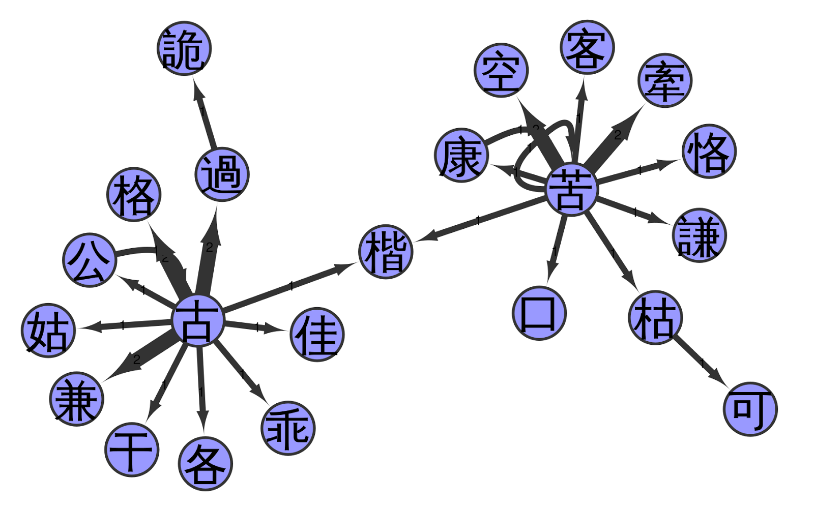
For example, based on the spellings reported in the Qièyùn, an early rhyme book published in 601 AD, we can say that the characters gōng 公, 古, gàn 干, etc. were regularly used to indicate initials that would be spelled as [k] in the International Phonetic Alphabet, while kǒu 口, 可, and 苦 were used to pronounce [] (a k with strong aspiration).

What I find even more interesting and important than these concrete findings, is that Chinese scholars inherently employed rudimentary network thinking to arrive at their clusters (Gēng 2004). The system of glossed character and glossing character can be easily translated into a system of directed networks, in which we draw a link from the glossing character to the glossed character.

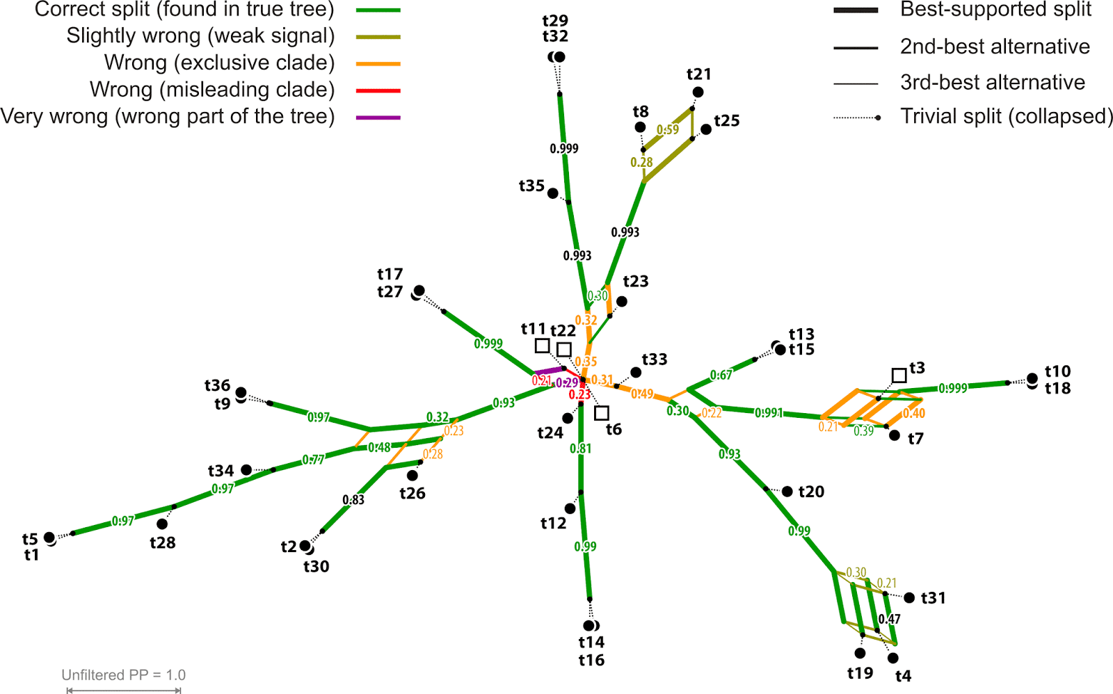
For a talk held earlier during the last year (List 2017), I constructed such a network from the Guǎngyùn (ca. 1000 AD), a later edition of the aforementioned rhymebook Qièyùn, which gives fǎnqiè spellings for more than 20,000 characters. In this network, I concentrated only on the initials, that is, the initial consonants of the language encoded in the source, and constructed a network of all internal relations among the glossing characters. The full network is shown in the following figure.


Eyeballing the network, we can see that the system does look rather systematic. The network is not connected and, apart from a few large connected components, we find a lot of discrete groups that seem to reflect individual initial sounds that were clearly distinguished from other sounds in the fǎnqiè spellings.

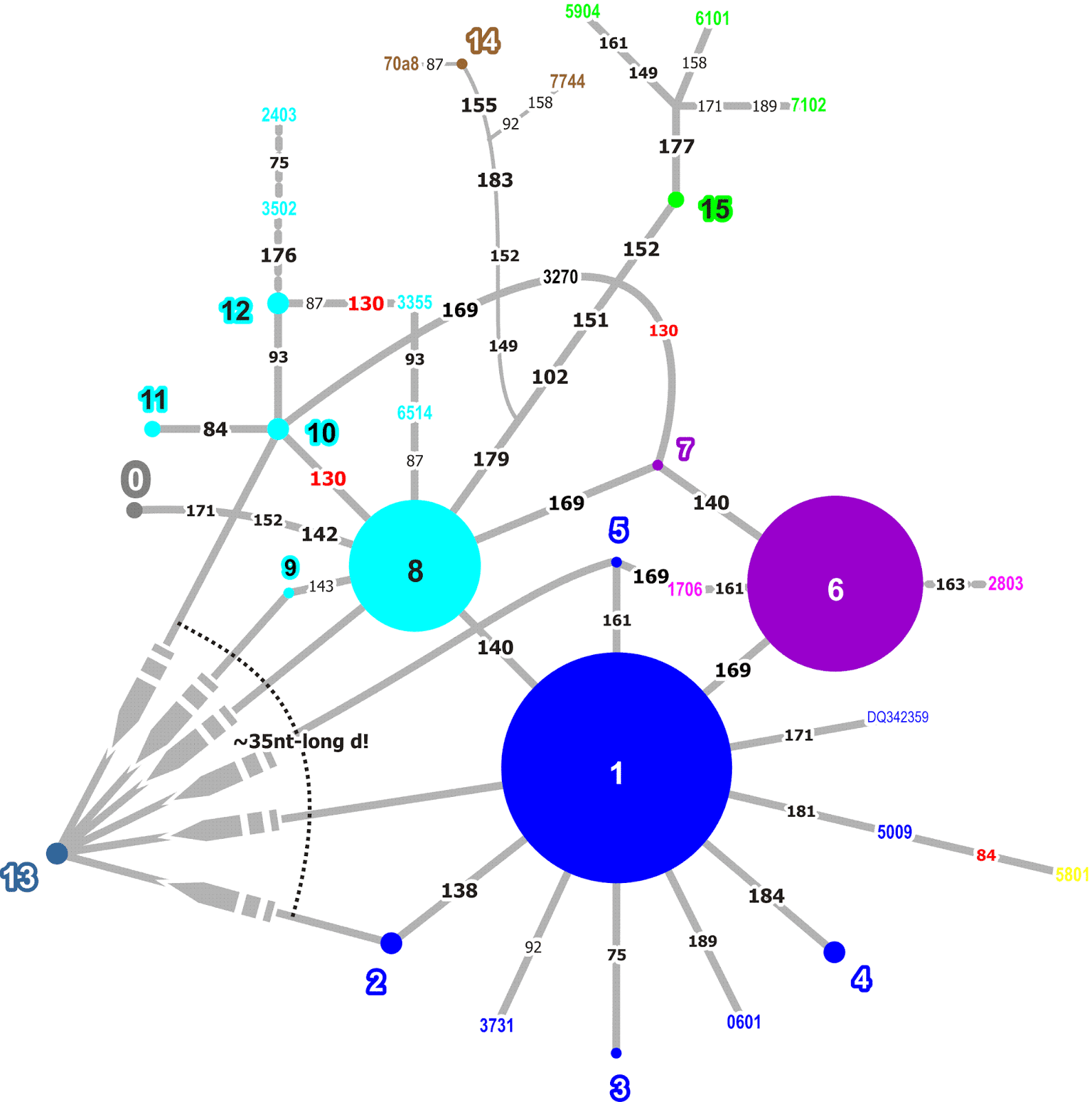
The following figure shows a part of the network, namely the second cluster in the big network (above) when going from left to right and staying at the top. In this figure, we can see that the network has two highly connected source characters linking to almost all of the other characters.


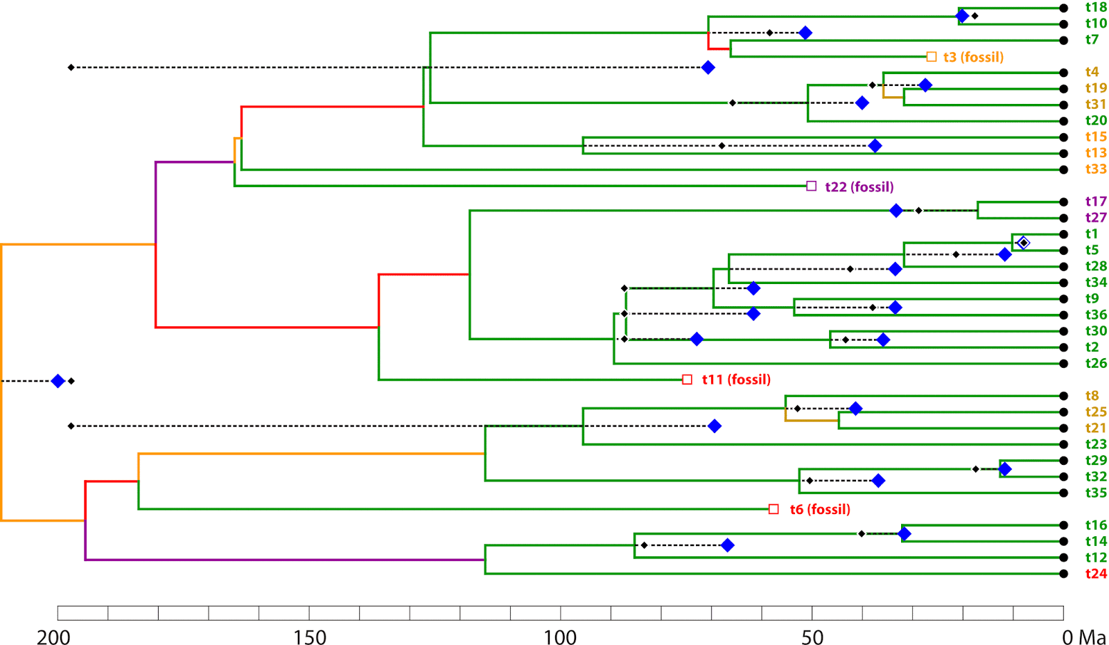
I have to admit that I am still having trouble interpreting the network satisfactorily, let alone designing more complex methods to analyse it. Nevertheless, I have the hope that the network analysis of Chinese pronunciation glosses can give us new insights into the phonetic history of Chinese. Importantly, the structures reflected by the network are true pronunciation differences, and that we can indeed find concrete sounds in the indirect fǎnqiè spelling system, becomes specifically clear when comparing the reconstructed pronunciations of the characters in the sample with each other.

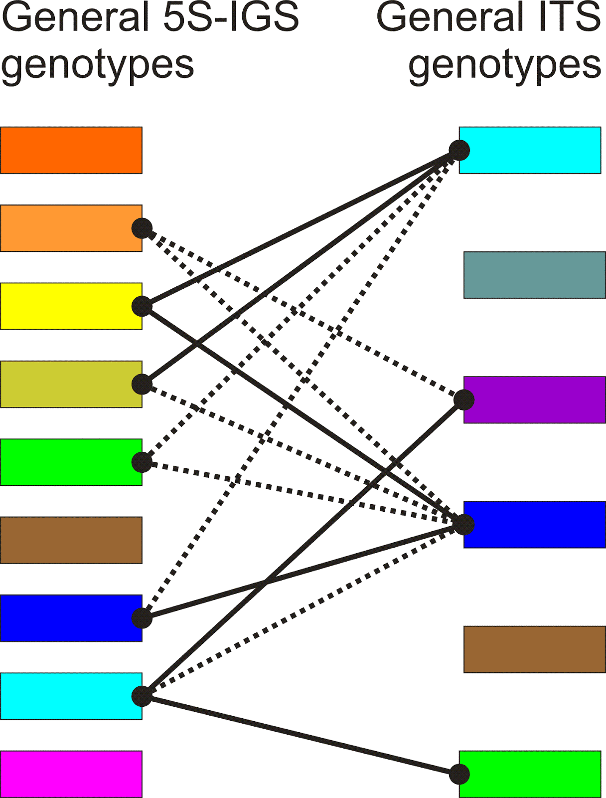
For example, when you look at the figure below, you can see that our connected component represents two different clusters of initials, namely a simple k and an aspirated . The node that links the two groups is given the pronunciation in our example, but its original reading is ambiguous. The character has two readings and two meanings reflecting both ancient k and ancient (today pronounced as jiē «Chinese pistachio tree» and kǎi «template», respectively).


Networks of pronunciation glosses in Chinese Traditional Phonology are still under-explored, both with respect to traditional scholarship and with respect to the way they are best handled and analyzed in modern network approaches. If we could develop an approach that would infer the clusters of glosses that point consistently to the same sound, they could give us fascinating insights, not only into the phonological system of Chinese varieties spoken during a given time period, but perhaps also into the dynamics underlying pronunciation changes, when comparing different networks across different times and places.

References
  • Branner, D. (2000) The rime-table system of formal Chinese phonology. In: Auroux, S., E. Koerner, H.-J. Niederehe, and K. Versteegh (eds.): History of the language sciences.1.18. de Gruyter: Berlin and New York. 46-55.
  • Coblin, W. (1983) A Handbook of Eastern Han Sound Glosses. The Chinese University Press: Chicago.
  • Gēng Zhènshēng 耿振生 (2004) 20 shìjì Hànyǔ yǔyīnxué fāngfǎ lùn 20世纪汉语音韵学方法论 [20th century’s methods in traditional Chinese phonology]. Běijīng Dàxué 北京大學: Běijīng 北京.
  • International Phonetic Association (1999): IPA Handbook. Cambridge University Press: Cambridge.
  • Kalusky, W. (2017) Die Transkription der Sprachlaute des Internationalen Phonetischen Alphabets: Vorschläge zu einer Revision der systematischen Darstellung der IPA-Tabelle. LINCOM Europa: München.
  • List, J.-M. (2017) Network approaches to the reconstruction of Old Chinese phonology. Talk, held at the "Center for Chinese Linguistics" (2017/03/07, Hong Kong, The Hong Kong University of Science and Technology).

Monday, January 22, 2018

Using median networks to understand evolution of genera


Median networks and their derivatives, such as median-joining and reduced median networks, are frequently used when studying genetic patterns within species. Indeed, this is what they were originally designed for. But occasionally, researchers have used them one taxonomic level up, to illustrate inter-specific relationships. For this blog post, I have dug out some reconstructions I made that I found quite interesting in this regard (including one that made it into publication), which I will discuss as examples.

Genetic markers

When working at the tips of the Tree of Life, where it becomes quite bushy, the messiness of species and permeability of species boundaries is one important issue. But another one is that we lack suitable genetic markers to collect data — we need gene regions that are variable enough to elucidate both intra- and inter-species differentiation patterns using tree inference.

One all-time classic marker is the nuclear-encoded ITS region, but this can be a multi-edged sword. Nuclear genomes usually include thousands of tandemly arranged repeats of the 35S rDNA, which includes the ITS region, in what is called the Nucleolus Organizer Region (NOR). The repeats may or may not be homogenized via concerted evolution. Furthermore, quite a few plants have more than one NOR, so we are dealing with paraloguous ITS sequences – in the strict genetic sense, these are sequences amplified from different loci (and chromosomes). In polyploids, we have ITS homoeologues passed on from the original donors. For instance, grasses can have four homoeologue NORs and ITS sets (usually adressed as "paralogues" in phylogenetic literature).

Even when not struggling with multiple ITS variants (intra-genomic variation), we can see the backside of concerted evolution: low ITS divergence in not a few plant genera. When ITS doesn't provide enough signal, researchers sometimes sequence the 3' end of the supposedly more variable 5'-external transcribed spacer of the 35S rDNA, the 5'-ETS (or just "ETS"). As an important terminological note: it is the 5'-ETS because there is another ETS at the end of the 35 S rDNA cistron, the 3'-ETS (essentially unknown except for organisms where the entire nuclear rDNA tandem repeat has been sequenced). Sequences uploaded to gene banks usually show the (repeat-free, or repeat-poor) 3' half and not the entire 5'-ETS, which has confused more than one researcher / reviewer — most but not all 3'-ETS sequences stored in gene banks are 5'-ETS.

When it comes to plastids, the currently best-covered most-variable marker is the trnH-psbA intergenic spacer, which includes prominent length polymorphic sections, which can be tricky to align once we go above the genus level (sometimes even within genera). The old plastic classic, the trnL/LF region, including the trnL intron and downstream trnL-trnF spacer, is probably the most sequenced plastid gene region; but it is usually too conservative to resolve even distantly related species of the same genus. Recently, many other alternatives have been recruited, thanks to completely sequenced plastomes.

Traditional intra-generic studies infer trees that often lack support at crucial branches, for two reasons:
  1. The authors overlooked (or ignored) incongruent signal from the combined gene regions (you wouldn't believe how many ITS-trnL/LF-backed published trees are fundamentally flawed);
  2. Many branches are supported by a single or very few mutational patterns (which is one reason why you see still a lot of cladograms in such studies, rather than phylograms showing the branch lengths).
Reason 2 does have a benefit, however — you may have unambiguous support for a branch collecting individuals (species) that are virtually identical.

Why median-networks?

When we are very close to the leaves of the Tree of Life, we work with faint primary signals, and often face very flat likelihood surfaces of the (inferred) tree space. When the rate of change is low, parsimony can out-compete probabilistic methods, in the sense that the inferred trees (or networks, as we will see below) are more informative. Median-networks apply the parsimony principle to reticulating relationships. However, in contrast to parsimony-optimized trees, (full) median-networks:
  • include all equally parsimonious solutions to explain the data;
  • can place taxa at internal nodes (the medians) — they can treat a sequence as ancestral to another.
Nevertheless, all species are contemporaneous, so they can't be each other's ancestors, right? Theoretically yes, but in reality, they actually can. When inferring species trees, we ignore the idea that one species may actually represent the remainder of an ancestral (paraphyletic) species after one (or more) populations became isolated. So, one living species can appear to be ancestral to another.

Another important point is that each (intra)specific lineage may have evolved at a different pace. We may thus find sequences in modern species that are much more primitive than are those of others (genetic "symplesiomorphies", if you want). The most striking example of a genetic symplesiomorphy that crossed my path was a 200-nt 18S fragment sequenced from a seedling found in a sea-locked cave. The people who sequenced it found best-BLAST hits with "basal" angiosperms, which didn't fit their matK fragment. This result was confirmed by re-sequencing, so they asked me to look at the data. I readily saw that the 18S fragment is from a core region, virtually identical across quite a range of angiosperms, including the group with a matching matK sequence. The ITS then showed that the matK's identification of the order (Myrtales) was correct, and that it was a Syszygium.


Fig. 1. A (reduced) phylogeny of Hoya (wax plants); one of the many intra-generic trees I inferred. Several unchallenged clades emerged (collapsed) as well as low-supported branches (grey backgrounds). A bootstrap consensus network revealed that the low support relates to semi-(in)congruent signals from the underlying matrix (including ITS, 5'-ETS, trnT-trnL, and trnL/LF data; see this post why you don't find this and the following graphs in the finally published paper: Wanntorp et al. 2014)

Example 1: Hoya

In the above tree (Fig. 1) the low support partly relates to incongruent nuclear and plastid signals from 'rogue' OTUs — these may be species / individuals, but it's typically just one individual per species. However, in other cases the signal from either the nuclear or the plastid data is simply ambiguous (not contrasting with the other part of the data) or semi-(in)congruent — the general affinity is the same but when it comes to exact placement, the nuclear data supports a different topology than the plastid data (Fig. 2).


Fig. 2. Maximum-likelihood bootstrap consensus networks for the complete plastid (A; trnT-trnL; trnL/LF) and nuclear (B; ITS + 5'ETS) data sets. Clades labelled only in one graph have little support (BS < 20) based on the other data. For example, there is no plastid counterpart to nuclear clades N and O, the taxa are scattered within the (cp-)H clade (but compare with Fig. 1! Pure data combination magic: strong support + ambiguity = equal or stronger support).

The failure to resolve e.g. the proximal relationships within the red clade and its relationship with respect to the blue clade and several minor clades (isolated OTUs) coloured pink in Fig. 2 (or resolution issues within the yellow-greenish bunch) has indeed to do with ambiguous signals due to less- and more-derived sequences.

Fig. 3. (Filtered) median-joining networks for each gene region. The graphs depict which clade has distinct (unique) sequence patterns, and can be interpreted regarding the potential evolution of the analysed gene regions. High(er) divergent markers: A, ITS1; B, trnT-trnL; low divergent markers: C, ITS2; D, trnL intron; E, trnL-trnF spacer.

At the genus level, these data are quite divergent (hence the tree in Fig. 1), and applying a median-joining network (or even reduced median) is computationally not feasible. So, in order to put their sequence variants into perspective, I filtered all group-specific site variations from the gene regions (singleton and unique mutations found only in a few members of a clade, or shared by a single OTU per clade, clade-unspecific stochastic convergences, are not considered). The complete data (raw and tabulated) can be found at figshare (Grimm 2017).

We can make some interesting observations. The pink species, OTUs attracted equally to the red and blue clades, have essentially underived or less derived sequence variants, either shared with or ancestral to the sequences of the red and blue clades. This applies to a more general degree also to the white species, highly ambiguous OTUs with no clear affinity to one of the major clades. The lack of unique shared genetic traits with any differentiated clade is the reason they are placed within the poorly supported, root-proximal ("basal") part of the tree(s).


Fig. 4. A tanglegram of the all-OTU plastid (left) and nuclear trees. Colouring as above (black font equals white in Fig. 3)

Another thing is that we can see that neither the main sequence features of clade III or IV, compared to clade V and VI, are consistently more primitive than their sister. They are proper sister clades that evolved from a common origin, but not from each other (via "budding"). This is something not obvious from the inferred trees (see Fig. 4). The pink sequences, scattered across the root-proximal ("basal") parts of the clade including pink, red, and blue OTUs are closer to the common ancestor shared with V (blue) and VI (red), but are obviously isolates from a first radiation round (note their position in Fig. 3A, D vs. B, C, and E and Fig. 4).

Example 2: Indomalayan and Australasian Ixora

This is a classic example of using median networks.

Ixora is a genus of Rubiaceae with a wide distribution in the tropics and subtropics of the Old World. As in the case of Hoya, I was recruited for the Banag et al. (2017) paper because the genetic differentiation patterns were very promising, but eluded the limited capacities of traditional tree inference.

The focus of the study was to find out how the high diversity of the genus in the Phillipine archipelago fits into the general framework of the genus. In contrast to Hoya (example 1) there is a (single) deep, well-supported incongruence between the nuclear (ITS, 5'-ETS) data set and the plastid data set (rps16 intron and the entire trnT–F region, as in the case of Hoya).


Fig. 5. Nuclear-plastid tanglegram for our Ixora dataset (Banag et al. 2017, fig. 1) Nuclear clade III is not found in the 'best-known' ML tree, but of the bootstrap (BS) sample preferred alternative (never ignore the BS consensus networks [nuclear/plastid], when facing low-supported branches in trees!)

In Ixora, we dealt with a number of main clades showing different nuclear-plastid combinations: I/A – red; I/B1 – orange; II/B2 and II/B3 – green; III/C – blue; IV/B (cultivars, not included in Fig. 5, showed additional combinations). Geographically, this leads to a compelling pattern (Fig. 6).


Fig. 6. Geographic maps of the genotyped samples (Banag et al. 2017, fig. 4). A. Nuclear data, B. Plastid data.


But to really trace the geographic-evolutionary sources of the highly diverse Philippine species set, which included members of nearly all lineages (except for the Afro-indian III/C), we had to deal with coherent but very few mutational patterns in the plastid gene regions. In contrast to the spacers of the 35S rDNA, plastid signatures are inherited maternally. Seeds often (but not always) travel less distance than pollen, and hence plastid differentiation in plants reflects primarily provenance. With respect to the low divergence, (nearly unfiltered) median-joining networks were a natural choice. Fig. 7 shows the close-up on the Philippines with the relevant plastid-based networks.


Fig. 7. Plastid-based median-joining (haplotype) networks for Ixora and their geographic distribution across the Philippine archipelago (Banag et al. 2017, fig. 5).

One observation here is that the trnTL reflects the isolation of the green species on Palawan (the island to the left), which tectonically is not a part of the Philippines. On the other hand, the trnLLF and rps16i of the green (dark green) species in Philippine proper derive from that of their Palawan counterparts, reflecting a stepwise colonization by the green lineage.

We also note that the red haplotypes representing lineage I/A unique to the Philippines are derived in comparison to the main purple type found all across the larger region, hinting towards a relatively long isolation time. This explains the topology of the plastid-based tree (Fig. 5) and its resolution issues. The purple haplotypes don't form distinct clades, because they are sequentially intermediate between the distinct sister clades (I/A, I/B1) and the equally widespread green lineage (IV/B2,B3).

Example 3: Western Eurasian species of Quercus subgenus Cerris section Ilex ('Ilex oaks')

This is a much more "beyond the edge" example of using median networks.

Differentiation patterns in the multicopy tandem-repeated nuclear spacers can be extremely challenging. In Göker & Grimm (2008) and Potts et al. (2014) we proposed network-based and network-affine methodological frameworks for how to deal with it. However, I did also explore the potential of median networks and their derivatives when applied close to the species level.

One particularly puzzling case is the species aggregate of Quercus aucheri, Q. coccifera, and Q. ilex, a group of wide-spread Mediterranean oaks (see also Simeone et al. 2016, and Vitelli et al. 2017 including median-joining networks). Q. ilex-type oaks have been co-dominant elements of the Mediterranean flora long before the Mediterranean became summer-dry (Denk et al. 2017).

For a never-published detailed study of Moroccan Q. ilex, I generated (essentially unreduced) median networks (following the protocol of Bandelt, Macaulay & Richards 2000) for two data sets of cloned ITS and 5S-IGS sequences, capturing intra- and inter-individual variation in the species and its sister species. 5S-IGS refers to the non-transcribed intergenic spacer of the 5S rDNA tandem repeats, a gene cluster delocalized from the NOR in most modern seed plants (in Ginkgo, for example, it's still located in the non-transcribed spacer between two 35S rDNA cistrons). As far as studied, oaks can have one or more loci per haplome encoding for the 5S rDNA repeats (and NORs; Ribeiro et al. 2011).

The main reason for this work was that I wanted to define ITS and 5S-IGS genotypes ("ribotypes") and to see how they map proportionally. The median networks appear quite complex at first sight (and possibly second and third, as well, when you are not the one who made them). Fig. 8 shows the median network for the 5' ITS1, which is the part of the ITS that sticks with the 18S pre-rRNA during the rDNA maturation process.


Fig. 8. A non-reduced median network for the 5' half of the ITS1 of western Eurasian Quercus ilex. Genotypes occurring in more than a single clone are coloured and numbered (1–15), coloured 4-digit numbers refer to individual clones (singletons), numbers at edges refer to the nucleotide site in the alignment showing the mutational pattern (convergent mutations in red font).

The mutational pathways don't seem to be overly complex, and the same holds for the other two non-coding, transcribed parts (functionally speaking) of the ITS region (3'-ITS1 and ITS2) and the 5S-IGS (Fig. 9).


Fig. 9. A non-reduced median network for the 5S-IGS data. Abbreviations refer to geographic regions, everything else as in Fig. 8 (the colours indicate no relation across the two figures)

Using such reconstructions as a basis, it is possible to make pie charts reflecting the frequency of the so-defined main genotypes (those with identical colours in Figs 8 and 9), and put them into a simple correlation graph (Figs 10, 11).


Fig. 10. Pie charts summing up the frequency of ITS genotypes (cf. Fig. 8) per geographic region/place.


Fig. 11. Correlation between 5S-IGS (Fig. 9) and ITS genotypes. Types with no links refer to individuals only covered for one of the data sets (thanks to the go-abroad policy of the German Science Foundation when becoming too good, I could not apply for a new project and had to leave the country, hence, lost my technician and lab and any possibility to fill the gaps)

Take-home message (actually: a call)

If you have data suitable to make median networks such as
  • overall low divergence
  • slow rate of change
or other beneficial situations for doing parsimony analyses, just give it a try. The more papers that are published showing such results, the easier it will become to get them past the confidential peer review. They can be a most versatile tool to understand molecular evolution, and the prospects and perils in our inferred trees, or competing support patterns (if you're already beyond tree-thinking).


There are further avenues that could be explored using the median network family. I already pointed out in an earlier post that they can depict the true tree when it comes to morphological data of modern-day taxa and their potential ancestors.

Another interesting thing would be to apply them to above-genus data sets when dealing with (very) slow evolving gene regions such as the 5.8S rDNA. For instance, backed by networks (median or others), one can see that the highly similar 18S rDNA of Juglandaceae and Myricaceae is likely a genetic plesiomorphy (which is one reason for the ambiguous support in oligo-gene Fagales trees).

Links

Download page for NETWORK, the free-software package I used to generate all of the median networks — http://www.fluxus-technology.com/sharenet.htm

What I was not allowed to show in #2: Networks explaining molecular evolution in wax plantshttps://researchinpeace.blogspot.fr/2017/12/what-i-was-not-allowed-to-show-2.html

(If you have more links, feel free to comment/contact: Let's make median networks great again #MeNeGA)

References

Banag CI, Mouly A, Alejandro GJD, Bremer B, Meve U, Grimm GW, Liede-Schumann S (2017) Ixora (Rubiaceae) on the Philippines – crossroad or cradle? BMC Evolutionary Biology 17:131.

Bandelt H-J, Macaulay V, Richards M (2000) Median Networks: speedy construction and greedy reduction, one simulation, and two case studies from human mtDNA. Molecular Phylogenetics and Evolution 16:8-28.

Denk T, Velitzelos D, Güner HT, Bouchal JM, Grímsson F, Grimm GW (2017) Taxonomy and palaeoecology of two widespread western Eurasian Neogene sclerophyllous oak species: Quercus drymeja Unger and Q. mediterranea Unger. Review of Palaeobotany and Palynology 241:98-128.

Göker M, Grimm GW (2008) General functions to transform associate data to host data, and their use in phylogenetic inference from sequences with intra-individual variability. BMC Evolutionary Biology 8:86.

Grimm G. 2017. Over-the-edge tables and reconstructions linked to the slimmed-down paper of Wanntorp et al. (2014), published in Taxon. figshare. https://doi.org/10.6084/m9.figshare.5688181.v1

Potts AJ, Hedderson TA, Grimm GW (2014) Constructing phylogenies in the presence of intra-individual site polymorphisms (2ISPs) with a focus on the nuclear ribosomal cistron. Systematic Biology 63:1-16.

Ribeiro T, Loureiro J, Santos C, Morais-Cecílio L. 2011. Evolution of rDNA FISH patterns in the Fagaceae. Tree Genetics and Genomes 7:1113–1122.

Simeone MC, Grimm GW, Papini A, Vessella F, Cardoni S, Tordoni E, Piredda R, Franc A, Denk T (2016) Plastome data reveal multiple geographic origins of Quercus Group Ilex. PeerJ 4:e1897.

Vitelli M, Vessella F, Cardoni S, Pollegioni P, Denk T, Grimm GW, Simeone MC (2017) Phylogeographic structuring of plastome diversity in Mediterranean oaks (Quercus Group Ilex, Fagaceae). Tree Genetics and Genomes 13:3.

Wanntorp L, Grudinski M, Forster PI, Muellner-Riehl AN, Grimm GW (2014) Wax plants (Hoya, Apocynaceae) evolution: epiphytism drives successful radiation. Taxon 63:89-102.

Monday, January 15, 2018

Tattoo Monday XIII — Bird trees


It's been nearly 3 years since we last had a tattoo blog post (see the list on the Tattoos page), and a few things have happened in the tattooing world since then. For today's post, here are some quite innovative ideas about a "Tree of Life" involving birds.


For those of you who are interested, Pinterest also has a page entitled "Tree of life tattoo", with quite a selection of images.

Tuesday, January 9, 2018

False reports of US women's breast sizes


The role of the social media in spreading fake news has recently been in the headlines; and it is becoming recognized as a major global risk, unique to the 21st century (the first known examples apparently date from 2010). For example, Chengcheng Shao et al. (The spread of fake news by social bots) note:
If you get your news from social media, you are exposed to a daily dose of false or misleading content - hoaxes, rumors, conspiracy theories, fabricated reports, click-bait headlines, and even satire. We refer to this misinformation collectively as false or fake news ... Even in an ideal world where individuals tend to recognize and avoid sharing low-quality information, information overload and finite attention limit the capacity of social media to discriminate information on the basis of quality. As a result, online misinformation is just as likely to go viral as reliable information.
However, an equally problematic issue occurs when the professional media indulge in the same practice — disseminating fake news online. A good example of this appeared during June-July 2016. It involved the presence online of this so-called research paper:
Scientific analysis reveals major differences in the breast size of women in different countries. The Journal of Female Health Sciences.

On the face of it, the paper seems very doubtful:
  • The concept itself is preposterous — although different genetic groups might have differences in breast size, on average, many countries have a mix of difference genetic groups, and thus should have a mix of breast sizes. There isn't an Olympics of breast dimensions!
  • The paper first appeared online in mid 2015, at a location not directly associated with any known journal.
  • The alleged journal's home page contains no references to any other published papers, nor to any mechanism for accessing or subscribing to it.
  • The alleged society publishing the journal has no internet presence, other than the journal homepage.
  • The alleged institutions from which the authors hail have no internet presence, other than the paper.
  • The alleged authors also have no internet presence, other than the paper.
It thus takes only a few minutes of effort to confidently identify this paper as a hoax. One therefore has to wonder why so much of the professional media did not make this effort. Instead, they enthusiastically listed the results, which proclaim the USA as having women with the largest breast size, on average, and the Philippines as having the smallest.

A Google search results in 755 hits to the paper's title, many of them internet commentaries. However, consider the following list of professional publications that took the paper seriously in mid 2016:
  • The Sun — The breast in the world: the countries where women have the biggest natural boobs in the world … and the smallest
  • The Telegraph — US women have the biggest breasts in the world — study reveals
  • The Mirror — The countries boasting the women with the biggest natural boobs revealed - where does Britain rank?
  • Daily Mail — Land of the free and home of the busty! American women revealed as having the biggest natural breasts in the world, while Brits come in fifth and Filipinos are last
  • The Irish Sun — Women in Ireland have the third biggest natural boobs in the world
  • New York Daily News — Red, white and boobs: American women boast the biggest breasts in the world
  • Seventeen — American women apparently have the biggest boobs in the world
  • Teen Vogue — U.S. women have the biggest boobs in the world, says science
  • FHM — Pinays have the smallest breasts in the world, study finds
  • Philippine Star — Study: Filipino women have the smallest breast size in the world
  • ABS-CBN — Study: PH women have smallest breasts in the world
  • South Africa Times — Where boobs grow biggest
Importantly, there were a number of commentators who did point out the hoax almost immediately the news reports started appearing:
  • Media Equalizer — Fake breast size study fools publications around the world
  • Manila Times — Fake research on women’s breast sizes is trite and boring
  • Daily Caller — Study showing America has world’s biggest boobs is a hoax but let’s rejoice anyway
  • Jose Carillo — Open letter on news stories that Filipinas have the world’s smallest breasts
Why, then, has the data subsequently been taken seriously in these places:
  • Radiation Oncology Journal 35: 121-128 (2017 ) In vivo dosimetry and acute toxicity in breast cancer patients undergoing intraoperative radiotherapy as boost.
  • Answers.com — Which country's women have biggest breasts in the world?


It is instructive to look at whether the perpetrators went to any trouble to produce their data. We can do this with a phylogenetic network, as usual on this blog. The network above is a NeighborNet based on the Euclidean distance — countries near each other in the network have similar breast sizes, and the further apart they they are then the less similarity they have. Only the 20 largest breast sizes are labeled.

You can see that the biggest breast sizes come preferentially from women with European backgrounds. You can also see just how extreme the breast sizes are claimed to be in North America. Both claims are actually doubtful.

Obviously, I do not know the origin of the paper and its data, but there is a somewhat similar presentation dating from March 2011, this time with a world map of bra sizes:
  • Target Map — Average breast cup size in the world
No source is identified for the latter data, but note that, in this case, it is the Nordic countries plus Russia that are reported to have the largest bra sizes. Indeed, the Spearman rank correlation between the the paper and map bra-size datasets is 0.71, so that only 50% of the variation in data is shared between the two datasets.

Finally, if you really do feel the need to read a scientific report about female breast morphology, then try this real one, which at least makes sense:
Evolution and Human Behavior 38: 217-226 (2017) Men's preferences for women's breast size and shape in four cultures.

Tuesday, January 2, 2018

Summarizing non-trivial Bayesian tree samples for dating? Just use support consensus networks


In a recent paper published in Systematic Biology, Joseph O’Reilly and Philip Donoghue (2017) shed some light on an issue concerning Bayesian analysis that has also bugged me since I first crossed paths with total evidence dating. Should we put dates on trees with topologies that may be “spurious”? Their answer is: "better not to". Based on their results, they advocate the use of majority-rule consensus trees (MRC), because maximum credibility clade (MCC) and maximum a posteriori (MAP) topologies may contain a critical number of erroneous branches.

I agree; but, being a notorious fan of non-trivial signals, in this post I will outline why one should generally use support consensus networks (SCN) to summarize the Bayesian tree sample, and then decide on those topological alternatives that are worth dating.

What O’Reilly and Donoghue found, and a simulation example

Using a series of simulated binary matrices and empirical datasets, these authors conclude that MCC trees, most commonly used by researchers doing total evidence (TE) or fossilized birth-death tip dating (FBD-TD), and MAP trees (rarely seen, but a reviewer asked the authors to include them, too) may contain too many erroneous branches (Fig. 1 provides an example). Low posterior probabilities are an alarm signal that should not be ignored. Being most conservative when it comes to accepting clades, MRC trees are hence less problematic.

Fig. 1 Tanglegram showing the true tree (left) in comparison to the inferred MCC tree.

But the problem naturally goes deeper: why can we have erroneous branches, and more importantly, low posterior probabilities?

When you have worked with a lot of messy datasets (ie. data with complex signal), you may have noticed that the optimized trees are not necessarily showing the best-supported splits. This also applies to ML optimizations, and molecular datasets (see example in my recent post). Morphological data are an especially challenging problem (post1/post2/post3/…). For the example in Fig. 1, the first of 10,000 MCCs O’Reilly and Donoghue inferred based on simulated data, it seems that:
  • all fossils are misplaced, some severely, but with consistently low support;
  • all deeper branches, branches near to the root, are (more or less) wrong.
A simple explanation for such a pattern is that the binary matrix is saturated, and hence shows a high level of homoplasy (like essentially all real-world morphological matrices). Later mutations (including many back mutations) overprint – to a certain degree – the signal of earlier mutations. How compatible are the signals from the matrix? Let’s take a look at the Neighbour-net and the matrix Delta value.

The prime problem: morphological data matrices provide no tree-like signals

With a matrix Delta value of 0.37, the matrix falls within the usual range seen in real-world morphological matrices, providing mainly non-treelike signals. The Neighbour-net (Fig. 2) is consequently boxy, with the central part approaching a spider-web — a very common structure when analyzing real-world morphological matrices. The Neighbour-net thus explains why the Bayesian MCC tree (and the Bayesian optimization in general) fails so miserably regarding some branches but not others.

Fig. 2 Neighbour-net based on mean morphological distances estimated from the matrix used for the Bayesian inference. Edge-bundles corresponding to branches in the true tree are highlighted in green.

The Neighbour-net includes several prominent edge-bundles matching more terminal relationships in the true tree. In these cases, the matrix provides strong, coherent signal, as also expressed in nearly unambiguous PPs. Some taxa such as t23, t24, and t33 provide quite ambiguous signals, and they are accordingly misplaced in the MCC tree — this is the reason for very low PP in the corresponding portion of the tree.

Regarding the fossils:
  • Tip-close fossil t3, an extinct sister lineage of clade {t7 + [t10+t18]} is clearly a close relative of the latter, which is something also resolved in the MCC (slightly wrong but with low support; Fig. 1) and MRC trees (where t3, t7, and t10+t18 would be part of a soft polytomy)
Root-close fossils (phylogenetically speaking) t6, t11, and t22 are harder to place
  • t11 seems to have some weak and misleading affinity to t17+t27 (compare with Fig. 1);
  • t6 is correctly placed in between clade {t12 + [t14+t16]} and clade t8–t35; and
  • t22 could be interpreted as an early side lineage of the latter clade (t8–t35), too, which is not too wrong with respect to its position in the true tree (but wrong in the MCC tree; Fig. 1).

Fig. 3 The topology of the MRC (Bayesian majority-rule consensus tree) in relation to the distance-based Neighbour-net.

Why consensus networks are without alternative

The standard MRC trees would collapse, to so-called “soft” polytomies, all of the erroneous branches in this example, plus a few correct ones (Fig. 3). This avoids the problem of misleading branches; but it comes with the cost that we cannot establish a sensible phylogenetic hypothesis and may even lose correct branches (four in the example). The 50%-MRC tree for the example in Fig. 1 would have 14 clades / terminals emerging from the soft root polytomy, which would leave us with (14-2)² = 144 topological alternatives — this is too many to consider. Consensus networks can reduce these options (Fig. 4). Plus, they inform us of whether a low support value is due to lack of discriminating signal or to conflicting signal. In the case of the simulated data, it’s naturally more the latter.

Fig. 4 SCN (support consensus network) based on 10,000 Bayesian sampled topologies (BST) O'Reilly & Donoghue inferred for their simulated data set Mk100/1.
Splits found in less than 20% of the BST not shown; trivial splits collapsed.
This sample was the basis for selecting the MCC (Fig. 1) and computing the MRC (Fig. 3) trees. Note how the soft polytomies in the MRC can be resolved into few competing alternatives.

Total-evidence can circumvent this problem to some degree, because the molecular data (in the optimal case) will constrain a backbone topology, which the morphological partition will have to fit into. Bayesian inference eliminates internal data conflict, as the chain optimizes towards a topology, or set of topologies, that best explain all data. This can have a streamlining effect on deep relationships, where the signal from the morpho-matrix is usually diffuse, but also towards the terminals. Here, the putative convergences conflicting with the molecular tree will be effectively down-weighted during the optimization.

Nevertheless, there are limitations. When the fossils show overall primitive or well-mixed character suites, there will be more than one possible placement. The consequence is topological ambiguity expressed in split support patterns. This is also the case for many fossils included in the dataset used in the original study introducing Bayesian TE dating (Ronquist et al. 2012), and as empirical examples in O’Reilly & Donoghue's assessment of MCC, MRC, and MAP trees.

Fig. 5 SCN (support consensus network) based on the 1000 last BST of both runs performed by O'Reilly & Donoghue on the full data set of Ronquist et al. (2012).
Blue edges refer to the branches seen in Ronquist et al.'s dated MRC tree (their fig. 7); modern-day groups and potential fossil members (open squares) coloured according to Ronquist et al. (2012: fig. 3). Filled circles: modern-day taxa. Note the prefential placements for a number of fossil taxa, which formed part of large, soft polytomies in the dated MRC tree. For instance, Palaeathalia, a fossil with highly ambiguous signal, is unresolved within the Tenthredinoidea clade in the MRC trees (emerges from a pentatomy, i.e. 52 = 25 principal topological alternatives). Based on the SCN, the number can be reduced to ten alternatives, which boiled down to three principal ones: sister to Tentredinidae, Blasticotomidae or all of Tenthredinoidea except for Blasticotomidae. The latter potentially including two additional fossils that are also part of the Tenthredinoidea pentatomy.

This is also the reason why we relied on fossilized birth-death dating for the Osmudaceae (Grimm et al. 2015). The earliest (Jurassic) representatives of the modern Osmundaceae (= Osmundeae according Bomfleur et al. 2017) that could be included in the total-evidence matrix shared many rhizome traits with the least-derived extant lineages (genera Claytosmuna and Osmunda; PPG I 2016). The signal from the morphological partition is not tree-like (see Bomfleur et al. 2015, fig. 8) and the total-evidence MRC accordingly collapsed with only the position of a single (unambiguous) rhizome fossil (Todea tidwellii) being fully resolved (Fig. 6).

Fig. 6 Total-evidence (TE) dating (Grimm et al. 2015) using the oligogene data by Metzgar et al. (2008; resulting in a fully resolved, unambiguously supported tree) combined with a morphological partition scording for rhizome traits of modern Osmundaceae (= Osmundeae according Bomfleur et al. 2017).
Four issues hinder the application of TE dating for this data set: 1. Poor backbone resolution (low, ambigous PP) preferring misleading relationships (cf. Bomfleur et al. 2015, 2017; Grimm et al. 2015). 2. The extant members of genera Claytosmunda, Osmunda, Plenasium are embedded in a large soft polytomy including fossils with the more primitive Claytosmunda-Osmunda rhizome morphologies. 3. Jurassic representatives of Osmundastrum (likely monophyletic) and Claytosmunda (paraphyletic according Bomfleur et al. 2017) form a poorly resolved "basal grade". 4. First representatives of Claytosmunda, Osmundastrum, and the Todea-Leptopteris lineage can be found in the Triassic, but cannot be included in a TE tree-inference framework (Bomfleur et al. 2017, fig. 15, section 2.2.3).
Fig. 6 (ctd) The results of fossilized-birth death datings that used only the frond (not used for TE dating) or rhizome fossils (same set than used for TE dating).
Osmundaceae foliage (sterile and fertile fronds) can be very characteristic and be traced in the fossil record, but provides only very few scorable traits. Shown chronograms modified from Grimm et al. (2015), supplement-fig. S2. Todinae: L. = Leptopteris, T. = Todea; Osmundinae: C. = Claytosmunda, O. = Osmunda, Om = Osmundastrum, P = Plenasium (cf. PPG I 2016; Bomfleur et al. 2017)


Shall we stop using TE dating?

Naturally, dating a MRC tree with large, deep polytomies (Figs 5, 6) will not be very revealing (Fig. 7). So, even though they are much less prone to error than MCC trees, they don’t provide a practical alternative. However, by using the SCN (support consensus network) we can:
  • depict the most likely (in a literal sense) topological alternatives (evolutionary scenarios); 
  • constrain their main aspects; 
  • date each of the resulting evolutionary scenarios; and 
  • compare the outcome. 
In the case of fast radiations, even fundamental changes to the constrained topologies will have little effect on the dating estimates (short branches)— even poorly resolved trees can provide age estimates that make sense (e.g. Grímsson et al. 2017). Really problematic involve only long(er) branches with poor support, preferred over equally or better supported alternatives.

Fig. 7 Variation in total-evidence dating estimates for the simulation example in Fig. 1 (O'Reilly & Donoghue's matrix Mk100/1).
The scale has been adjusted to fit the fossils' relative ages and assuming an actual (real) root age of 200 million years (Ma). Shown is the MCC chronogram, the estimates of corresponding nodes according to the equally scaled MRC tree (black diamonds), and the target divergence ages (blue diamonds) according to the true tree (the tree used to simulate the data). The saturation of the morphological partition triggers too long terminal branches in both the MCC and MRC trees, hence, most mid-topology estimates are overestimating. MRC-derived estimates can be better than MCC estimates, but also much worse due to collapsed soft polytomies. Note that in the case of real-world data, the molecular partitions may compensate for the branching-length bias to some degree (see also Fig. 6).

Furthermore, the SCN will point us to the ‘weak spots’ in our fossil-inclusive phylogeny, and also to the rogues — fossils with strongly ambiguous (non-treelike) signal that mess up any tree inference. For dating, we need a tree, and hence a set of taxa providing a tree-like-as-possible signal (see the reduced data set used in Ronquist et al. 2012 for the in-text figures). For all other data sets, where ambiguous signal from fossils and morphology is inevitable, the (original) fossilized birth-death dating remains the best option.

However, be careful with the new tip-dating option, because this again assumes that the position of fossils can be unambiguously optimized in the tree.

One thing is clear: (largely) ignoring the fossil record when doing molecular dating to infer organismal histories is the worst of all possibilities.

Thanks

To Joe O'Reilly for providing the Bayesian result files (BST samples, MCC and MRC trees) used in their study.


Related posts

Why we should use consensus networks to summarize Bayesian analysis:
Issues with node dating that may effect TE dating, too, and can only overcome by using the entire fossil record of a group (FBD dating
Non-treelike morphological data used to infer (strict) consensus trees:
Stacking neighbour-nets, a real-world example using the Osmundaceae matrix (matrices) of Bomfleur et al. 2017

References

Bomfleur B, Grimm GW, McLoughlin S. 2015. Osmunda pulchella sp. nov. from the Jurassic of Sweden—reconciling molecular and fossil evidence in the phylogeny of modern royal ferns (Osmundaceae). BMC Evolutionary Biology 15:126. http://dx.doi.org/10.1186/s12862-015-0400-7

Bomfleur B, Grimm GW, McLoughlin S. 2017. The fossil Osmundales (Royal Ferns)—a phylogenetic network analysis, revised taxonomy, and evolutionary classification of anatomically preserved trunks and rhizomes. PeerJ 5:e3433. https://peerj.com/articles/3433/

Grimm GW, Kapli P, Bomfleur B, McLoughlin S, Renner SS (2015) Using more than the oldest fossils: dating Osmundaceae with the fossilized birth-death process. Systematic Biology 64: 396–405.

Grímsson F, Kapli P, Hofmann C-C, Zetter R, Grimm GW (2017) Eocene Loranthaceae pollen pushes back divergence ages for major splits in the family. PeerJ 5: e3373. https://peerj.com/articles/3373/

Metzgar JS, Skog JE, Zimmer EA, Pryer KM. 2008. The paraphyly of Osmunda is confirmed by phylogenetic analyses of seven plastid loci. Systematic Botany 33:31–36.

O'Reilly JE, Donoghue PCJ (2017) The efficacy of consensus tree methods for summarising phylogenetic relationships from a posterior sample of trees estimated from morphological data. Systematic Biology https://academic.oup.com/sysbio/advance-article-abstract/doi/10.1093/sysbio/syx086/4587515

PPG I. 2016. A community-derived classification for extant lycophytes and ferns. Journal of
Systematics and Evolution 54(6):563–603 http://onlinelibrary.wiley.com/doi/10.1111/jse.12229/epdf

Ronquist F, Klopfstein S, Vilhelmsen L, Schulmeister S, Murray DL, Rasnitsyn AP (2012) A total-evidence approach to dating with fossils, applied to the early radiation of the hymenoptera. Systematic Biology 61: 973–999.