Median networks have been designed to put within-species haplotypes into an explicit evolutionary framework. They are exclusively parsimony-based, but differ from traditional trees by treating operational taxonomic units (OTUs) as both potential tips and ancestors. Ancestors are placed at internal nodes ('medians'). The latter makes them interesting for hypotheses about sequence evolution; but, like all parsimony-based methods, they suffer from high levels of homoplasy, which is a common feature of genetic data sets.
Can we use median networks to better understand evolution far above the species level?
In order to test this, I generated a median network using data on the nuclear-encoded 5.8S rDNA of Fagales. This is a flowering plant (angiosperm) order, which includes well-known trees such as oaks, beeches, chestnuts, walnuts, alder, birch and hazel, but also the enigmatic 'false beech' (
Nothofagus s.l., the traditional four subgenera have been elevated to genera by Heenan & Smissen 2013), a Gondwanan element that (for some time) has intrigued biogeographers.
Why I have always loved nrDNA
A a young (phylo-)geneticist,
my boss, a geneticist who sequenced genes such as the rRNA genes before PCR made it easy, pointed me to the works of Mark Hershkovitz, Louise Lewis, and Edith Zimmer about evolution
of the nuclear-encoded ribosomal RNA genes (nrDNA) in angiosperms. Long pre-dating the era of big data and self-evident, trivial phylogenies (ie. data sets allowing for the inference of a fully resolved, unambiguously supported tree), Hershkovitz and co-workers sought to extract as much information as possible from the best-known gene region available back then (mid-late 90s): the internal transcribed spacers (ITS1, ITS2) of the 35S rDNA, the cistron encoding the genes for the 18S, 5.8S and 25S (or 28S, but not "26S") nuclear ribosomal RNA.
- Hershkovitz MA, Lewis LA. 1996. Deep-level diagnostic value of the rDNA-ITS region. Molecular Biology and Evolution 13:1276–1295.
- Hershkovitz MA, Zimmer EA. 1996. Conservation patterns in angiosperm rDNA ITS2 sequences. Nucleic Acids Research 24:2857–2867.
- Hershkovitz MA, Zimmer EA, Hahn WJ. 1999. Ribosomal DNA sequences and angiosperm systematics. In: Hollingsworth PM, Bateman RM, and Gornall RJ, eds. Molecular Systematics and Plant Evolution. London: Taylor & Francis, pp. 268–326.
The ITS1 and ITS2 are highly divergent, non-coding but transcribed intergenic spacers within the structurally and sequentially much more conserved nrDNA, which distinguishes them from nearly all other non-coding regions. More often than not, their sequences are impossible to align across high-ranking taxa such as families or orders. The brilliance of Hershkovitz et al.'s work was to just go a level-up by identifying shared general sequence patterns, and to put them in an evolutionary context.
 |
| Birds-eye view of the ITS region (consensed for sequence groups) in Fagales including sequences of the two outgroups used in Li et al. 2004 (zoom-in and try to figure out where they are). The position of the ITS(1) cleavage site is indicated, a highly conserved, AT-dominated sequence motif within the ITS1. The "Nothofagus deletion" (Manos 1997), gray area seen in some of the topmost variants in the 5.8S rDNA, is a sequencing/ editing artifact (newer sequences all have a complete 5.8S rDNA). Most of these data are more than 15-years old (see references provided at the end of the post) and may include more data artifacts, especially in the length-polymorphic portions. Nonetheless, part of the data were included in the dating studies of Sauquet et al. (2012) and Xing et al. (2014) to compensate for the lack of resolution of the also included plastid regions towards the tips of the Fagales tree (intrafamily and -generic relationships). |
Accordingly, in my
(open access) Ph.D. thesis you'll find not a few figures depicting the potential evolution of sequence patterns in the ITS1 and ITS2 of maples and the beech trees.
I could probably write a book taking up where Hershkovitz et al. stopped, but this would be: a) very subjective, and b) too complex and marginal for the 21st century. Very few people would read it. We have grown accustomed to simple graphs as metaphors of evolution and, thanks to big data, we have become reluctant to discuss the results
ex machina. Also, I would have needed a score of students to pursue all the avenues that I glimpsed into; e.g. the following pic:
 |
| Evolution of the 5'-end of the ITS1 in basal eudicots (looking at divergences that happened, at least, 100 myrs ago). |
The other way around
If the more conserved sequence patterns within the ITS1 and ITS2 can be informative about evolution at a much higher level (which they are), the next question is: what can we learn from the sequence patterns in the highly-conserved portions of the rDNA linked with the ITS1 and ITS2? Historic-genetically, the ITS1 is fundamentally different from the ITS2. The former, ITS1, is an intergenic spacer, which has no secondary structure (although you can find reconstructions in literature) as it is split into two parts right after translation (the ITS1 cleavage site is quite conserved, and a main topic in the papers by Hershkovitz and Zimmer). The latter, ITS2, has been evolutionarily derived from the first variable portion of the large ribosomal subunit (LSU), the 25S (28S) rDNA. In primitive organisms, there is hence no 5.8S rDNA and ITS2.
This geno-evolutionary history is also the reason for the structural linkage between the 5.8S rRNA and the 5' end of the 25S (28S) rRNA. Here's a zoom-in on the part that we are interested in.
For better orientation, I have named some of the extremely conserved secondary structure elements of the (mature) 5.8S rRNA. Note that the "Gingerbread Man" structure is very conserved in angiosperm sequences although it only contains three very short stems. The "Pimple" and the "Needle" are so-called hairpins — a strictly complementary stem part is capped by a short, non-complementary tip ('semi-loop'): a 3- and 4-nt long motif, respectively, in
Arabidopsis and all Fagales (in some species of
Lithocarpus, the tropical 'stone nut' and relative of oaks, the "Needle" has two extra nucleotides).
5.8S rDNA in Fagales
I chose the Fagales because I have worked on them a lot, they are a pretty small group, and except for
one "asterisk branch" their inter-family relationships are solved.
 |
| Basic signal in Li et al. (2004)'s matrix. Inter-family relationships are, data-wise, fairly trivial, hence, the tree-like Neighbor-net. Only the placement of the Myricaceae with respect to Juglandaceae (now incl. Rhoipteleaceae) and Betulaceae + allies is not unambiguously resolved (see this post) |
Oaks have received a lot of attention from population geneticists, like other widespread species or species complexes. Those studies, using Median networks and related methods such as Statistical Parsimony, revealed very complex genetic diversity patterns. On the other hand, the Fagales lineage has been fairly neglected by plant phylogeneticists, although it comprises many of the dominant, ecologically and economically most important trees of the Northern Hemisphere (and the enigmatic Gondwanan Nothofagaceae). The early studies found evidence for deep nuclear-plastid incongruences, but only in recent years has the first (non-comprehensive) complete plastome phylogenies and dated all-Fagales trees surfaced (which do contain
one or other common error and
misinterpretation of results).
For one family, the southern hemispheric, tropical-subtropical Casuarinaceae, we have no
(reliable) ITS data at all; also missing is one of the genera of the Juglandaceae:
Engelhardia (s.str.; most data in gene banks labelled as
Engelhardia is from
Alfaropsis; cf. Manchester 1987 and Manos et al. 2007, but see Zhang et al. 2013).
In total, we find 17 variable sites at and above the genus level in the 5.8S rDNA of Fagales. There are three in the core parts, structurally linked to the 5' 25S rRNA, two in the 'Gingerbread Man', three in the 5' and 3' trails, and the rest are in the 'Needle'.
 |
| Unique mutations and mutational trends (arrows) in the 5.8S rDNA in Fagales. Circles highlight the basepairs differing from the reference (Arabidopsis 5.8S rRNA). Blue, mutations found within more than one major lineage, pink, lineage-conserved (diagnostic) mutations; red, mutations restricted to a single genus; green, genetic (syn)apomorphies of the 5.8S rDNA of Fagales. Be = Betulaceae; Ju = Juglandaceae; My = Myricaceae; No = Nothofagaceae; Fagaceae include Fagus (Fa, the beech) and the remainder ("Quercaceae": Qu), which are genetically substantially distinct from Fagus. |
Many mutations are genus-coherent; increased intrageneric variation is found in the 5'-tail and the part encoding the 4(6)-nt long 'semi-loop' sequence of the "Needle" (pos. 120–142 in the rRNA of
Arabidopsis thaliana):
 |
| A (near-)full Median network for the tip of the 'Needle'. In a few Lithocarpus (a "Quercaceae" genus) the sequence is 6-nt-long, which would result in an elongated hairpin (paired basepairs are underlined). The ATTC is a genetic symplesiomorphy. |
Exceptions are
Fagus and
Quercus, which can show substantial intra
genomic ITS divergence,
Lithocarpus (the most divergent genus, ITS-wise)
, and
Nothofagus s.l. (between the former subgenera, now genera). In these cases, the intra-(sub)generic variation includes the putatively ancestral nucleotide and/or nucleotide shared with other genera of the family; eg. at pos. 123, all Fagales have a C,
Fagus can have either C or T (= Y), and
Quercus can show any of the four nucleotides (= N).
A Median-network for the 5.8S rDNA
Ambiguities can be detrimental for resolution in standard parsimony implementations. The
NETWORK program, for instance, warns that a code of "N" may render the result less reliable, and this applies also to the other ambiguity codes. If we include the intra-generic polymorphisms as ambiguity codes, N
ETWORK runs for quite a long time: too many solutions are equally parsimonious (for this experiment I used genus-consensus data, being interested in the deep splits)
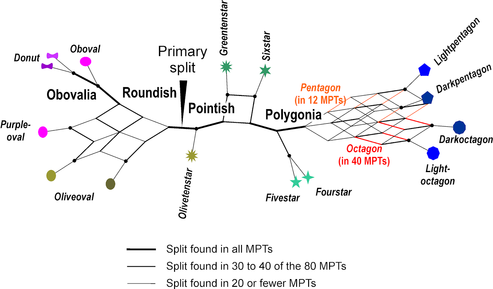
But when we resolve the intra-generic polymorphisms prior to analysis by treating them as satellite types, ie. assuming the family-shared nucleotide represents the ancestral state within the according lineage, we quickly get the following result:
 |
| Edges colored to trace the same mutational step. Bubbles indicate the position of the (basic) 5.8S rDNA genotypes for the genera in each family-level lineage. |
This is still not a too trivial graph, but it:
- provides a framework on which we can develop our evoluionary scenario;
- visualizes how mutational patterns may be linked;
- tells us directly how derived (genetically) and unique (isolated) the genera are.
Since the 5.8S rDNA is part of a multi-copy (potentially multi-loci, Ribeiro et al. 2011) gene region, uniqueness gives us an idea about how reduced a lineage is. Bottlenecks will eliminate intra-lineage diversity and unique mutational patterns are more likely to accumulate in a species-poor lineage with small population sizes.
But since it is a vital gene region underlying strong sequential and structural constraints, evolution is not neutral: the graph has little tree-likeness. However, the graph looks like graphs that one expects for fast ancient radiations.
There are more interesting details. For instance, we have no mutation separating consistently the earliest diverging lineages (given the currently accepted root), the Nothofagaceae and the Fagaceae (s.l.) and the remainder of the order (called "higher hamamelids" in classic systematic literature). We also see that the 5.8S rDNA shows the Fagaceae should be monotypic:
Fagus is more different from its siblings, the 'Quercaceae', than it is from the first-diverging Nothofagaceae or the common ancestor of the "higher hamamelids". Fagaceae s.str. and 'Quercaceae' are without a doubt sister lineages but this also applies to Betulaceae and Ticodendraceae (differing only by three point mutations), with the Betulaceae being just one point mutation away from its more distant sibling (phylogenetically speaking), the Juglandaceae. Furthermore, for
Ticodendron-Betulaceae we can postulate a sequentially unique common ancestor, but we can't do the same for
Fagus-'Quercaceae'.
Either the 5.8S rDNA evolved much faster in
Fagus than in most other lineages, or
Fagus split away from its sisters prior to the radiation of the "higher hamamelids" and shortly after their respective ancestors isolated. This second scenario coincides nicely to recent fossil findings tracing the
Fagus lineage back to the late Cretaceous (at least 80 Ma; Grímsson et al. 2016, supplement includes a digression of all-Fagales dating attempts).
Reconstruction of ancestral genepools
Using the split patterns in the network to extract an evolutionary tree could be hazardous, since we are looking at strongly interconnected mutational patterns filtered by selective pressure (maintaining a functional structure) in a gene region that evolves very slowly: some sites can or did accumulate mutations (the 'Needle' and the trails), others can't and did not (the remainder of the 5.8S rDNA) in the Fagales lineage. At least mutations were not fixed over a long evolutionary time: the data includes at least as many variable sites where within a single genus, species or genome, the shared, family-typical nucleotide (or even shared with
Arabidopsis, a quite distant relative of Fagales) is occasionally replaced.
But since we know the phylogeny of the Fagales, we can, based on the Median(-joining) network(s), infer the evolution of the 5.8S rDNA (i.e. the rDNA gene pool) over time:
 |
| Results of the Median-joining analysis mapped on the currently accepted Fagales tree. Clade-characteristic mutations are highlighted by according colors; black, homoplastic mutations that occurred independently in two lineages, gray, in more than two. |
Regarding the 'asterisk branch', the 5.8S rDNA provides few extra clues, unless we want to re-include a third hypothesis: that the Myricaceae are sister to Juglandaceae + Betulaceae and allies. This would be the most fitting explanation for the 5.8S rDNA diversity. It also would explain why they can be either sister to Betulaceae and allies or Juglandaceae. Ancestors, or slower evolving sisters diverging shortly before a radiation, will do such a thing.
In this context, one should point out that unequivocal fossils representing various modern genera of all families are known from the early Paleogene, many pop up in early Eocene (~ 50 Ma) intramontane basins of northwestern North America. The oldest modern genus and a possible living fossil is the first diverging Juglandaceae:
Rhoiptelea. Its pollen can be found from the Maastrichian onwards in North America and elsewhere, and a fossil showing the unique
Rhoiptelea-flower and fitting pollen can be found in the late Turonian-Santonian (~90 Ma) of Bohemia (Heřmanová et al. 2011; the authors, however, decided to name it
Budvaricarpus and tone down the striking resemblance to modern-day
Rhoiptelea).
Of course, since we use network-based approaches, we can conceptualize the 5.8S rDNA sequence patterns and inferred evolution as a subsequent breaking up and sorting of once-shared gene pools:
 |
| A 'coral' tree metaphor for the evolution of the 5.8S rDNA in Fagales (using an alternative, one-node-shifted root). |
I chose an alternative root because it is the one that makes most sense regarding the fossil-morphological, palaeoclimatological/-vegetation and high-conserved genetic patterns (thinking of the 18S rDNA). The labels are, of course, a gross simplification — it is likely that the all-ancestor was a tropical-subtropical plant as well (the genetically most unique and potentially earliest isolated genera of the 'Quercaceae' are exclusively tropical-subtropical) and Myricaceae, Betulaceae and Juglandoideae can today be found deep into the temperate zone, some even thriving in boreal and polar climates. But posts can afford to trigger discussion.
The vertical axis reflects not only the derivedness of the 5.8S rDNA, but also the potential sequence of divergences back in time. The horizontal axis represents the taxonomic-geographic breadth over time (very roughly, tapering means higher diversity/greater range in the past than today) and towards the tips the genetic within-lineage diversity seen in the ITS1 and ITS2 (in Myricaceae, it would be close to a point, if it would not be for one species:
Myrica gale, the bog myrtle or sweetgale, beloved in Scotland and Scandinavia – see this
Dane's video for how to use it).
Just a curious experiment?
Now, to most readers this post may just be a strange example with little general relevance for phylogenetics. But consider the following.
- When we infer deeper phylogenetic relationships, we usually rely on sequence differentiation in coding-gene regions. Like the rRNA genes, the tRNA genes need to fulfill secondary (and tertiary) structural constraints to maintain their vital functions. All other genes code for proteins, which also need to fulfill structural constraints (secondary, tertiary and quaternary structures). Their essential functions rely on keeping a specific amino-acid sequence, which is translated from DNA sequences.
- We do this inference under the assumption that molecular evolution is neutral, which, as can be seen in the case of the 5.8S rDNA, is apparently not the case. Mutations that would negatively affect the function of the DNA-transcripts are strongly selected against.
Many of our trees makes sense nonetheless, but we should keep a wary eye on all of those branches that draw their support from only one or two gene regions (a common issue of oligo-gene trees like the one by Li et al. 2004), or very few mutations. Especially, when we are producing an ultrametric tree. How sensible can a divergence age estimate be when the data behind it are four mutations in the monotypic lineage and zero in its more diverse sister clade?
Cited literature and further reading (with comments).
ITS studies (some mixed with further data and results that were ignored by all-Fagales dating studies that included the data)
- Acosta MC, Premoli AC. 2010. Evidence of chloroplast capture in South American Nothofagus (subgenus Nothofagus, Nothofagaceae). Molecular Phylogenetics and Evolution 54:235–242. See also Premoli
AC, Mathiasen P, Acosta MC, Ramos VA. 2012. Phylogeographically
concordant chloroplast DNA divergence in sympatric Nothofagus s.s. How
deep can it be? New Phytologist 193:261–275. — Just two brilliant papers that only leave one question open: is this different in the Australasian genera of the Nothofagaceae?
- Cannon CH, Manos PS. 2003. Phylogeography of the Southeast Asian stone oaks (Lithocarpus). Journal of Biogeography 30:211–226. — A very well-done paper that still doesn't need to fear to comparison with more recent biogeographic papers on Fagales genera with access to more elaborate inference methods, while using much poorer data samples.
- Denk T, Grimm GW. 2010. The oaks of western Eurasia: traditional classifications and evidence from two nuclear markers. Taxon 59:351–366. — Since this is mine, I should not give myself an assessment. Just some info: it was the most sloppy draft, we ever submitted, and passed rather smoothly the review process. But it used 600+ new ITS and 900+ new 5S-IGS sequences, and although it provided a comprehensive ITS tree (new and all data stored in gene banks), the conclusions relied mostly on networks based on inter-clonal and inter-individual distances and ML bootstrap pseudoreplicate samples. I'm pretty sure, it's still hard to find a similar paper.
- Denk T, Grimm G, Stögerer K, Langer M, Hemleben V. 2002. The evolutionary history of Fagus in western Eurasia: Evidence from genes, morphology and the fossil record. Plant Systematics and Evolution 232:213–236. — My first phylogenetic paper (using only about 100 ITS sequences) and one of my most-cited papers; published only because the editor ignored the opinions of two reviewers.
- Denk T, Grimm GW, Hemleben V. 2005. Patterns of molecular and morphological differentiation in Fagus: implications for phylogeny. American Journal of Botany 92:1006–1016. — the follow-up paper, including all beech species.
- Forest F, Bruneau A. 2000. Phylogenetic analysis, organization, and molecular evolution of the non-transcribed spacer of 5S ribosomal RNA genes in Corylus (Betulaceae). International Journal of Plant Sciences 161:793–806. — Likely the reason for the 2005 study by Forest et al., a great paper (especially when compared to other phylogenetic papers published in the same journal back then and much later). The reason why the 5S-IGS has rarely been studied, is because it is difficult to handle (usually one needs to clone because of intraindividual length-polymorphism). But it provides an unsurpassed resolution at the intrageneric level that only finds a match in the last years by the accumulation of NGS SNP data.
- Forest F, Savolainen V, Chase MW, Lupia R, Bruneau A, Crane PR. 2005. Teasing apart molecular- versus fossil-based error estimates when dating phylogenetic trees: a case study in the birch family (Betulaceae). Systematic Botany 30:118–133. — A pivotal, still valid study using ITS and 5S-IGS data, even though the divergence age estimates are probably much too old (an aspect demonstrating the quality of the study, back then, molecular age estimates were usually much too young). Forest and Bruneau published several other papers of equal quality on other plant groups, and I suspect there is an interesting publication story given the author list and the dissemination platform.
- Grimm GW, Denk T, Hemleben V. 2007. Coding of intraspecific nucleotide polymorphisms: a tool to resolve reticulate evolutionary relationships in the ITS of beech trees (Fagus L., Fagaceae). Systematics and Biodiversity 5:291–309. — A crazy experiment, but one that, years later, would bring me my first paper in Systematic Biology [PDF] (10-times higher impact factor) because it was the only piece of science providing a way-out for a young researcher in South Africa.
- Manos PS. 1997. Systematics of Nothofagus (Nothofagaceae) based on rDNA spacer sequences (ITS): taxonomic congruence with morphology and plastid sequences. American Journal of Botany 84:1137–1155. — A typical study for the time, may be not ground-breaking but opening an interesting path and still the basis for molecular systematics of Nothofagaceae (getting such data in the late 90s was not easy). Interestingly, no-one in Australia or New Zealand ever took the thread up (but see Knapp et al. 2005), the only only properly studied genus (then a subgenus) of Nothofagaceae is Nothofagus s.str. (Acosta & Premoli 2010; Premoli et al. 2012).
- Manos PS, Doyle JJ, Nixon KC. 1999. Phylogeny, biogeography, and processes of molecular differentiation in Quercus subgenus Quercus (Fagaceae). Molecular Phylogenetics and Evolution 12:333–349. [PDF] — The counterpart to the above for oaks, it took nearly two decades to assemble more data on American oaks than used for this study.
- Manos PS, Stone DE. 2001. Evolution, phylogeny, and systematics of the Juglandaceae. Annals of the Missouri Botanical Garden 88:231–269. — An exemplary paper for two reasons (and despite the fact that it just shows cladograms): 1) it combined morphological and chemotaxonomic data with ITS and plastid data (rbcL-atpB and trnL-trnF intergenic spacer); 2) pretty much got the still accepted tree. Also proof-of-point that, even 20 years ago, studies in low-impact journals were not rarely better than those in high-fly ones. (Note the number of pages; decent research needs space!)
- Manos PS, Zhou ZK, Cannon CH. 2001. Systematics of Fagaceae: Phylogenetic tests of reproductive trait evolution. International Journal of Plant Sciences 162:1361–1379. — For years to come the basis for Fagaceae systematics.
- Muir G, Fleming CC, Schlötterer C. 2001. Three divergent rDNA clusters predate the species divergence in Quercus petraea (Matt.) Liebl. and Quercus robur L. Molecular Biology and Evolution 18:112–119. — Only about two species, but setting the scene: ITS evolution in Fagales (and probably any other wind-pollinated tree) can be very complex at the very basic level.
- Ribeiro T, Loureiro J, Santos C, Morais-Cecílio L. 2011. Evolution of rDNA FISH patterns in the Fagaceae. Tree Genetics and Genomes 7:1113–1122. — A must-read for everyone using ITS data in Fagales.
Phylogenetic studies at and above family level
Betulaceae: see Forest et al. (2005) and Grimm & Renner (2013, following section).
Casuarinaceae: see 'Phylogeny' section on Stevens' Angiosperm Phylogeny Website (never bothered myself with them, since they lack ITS data).
Fagaceae: see Manos et al. (2001), tree in Denk & Grimm (2010)
- Oh S-H, Manos PS. 2008. Molecular phylogenetics and cupule evolution in Fagaceae as inferred from nuclear CRABS CLAW sequences. Taxon 57:434–451. — The molecular basis for Fagaceae systematics.
- Manos PS, Cannon CH, Oh S-H. 2008. Phylogenetic relationships and taxonomic status of the paleoendemic Fagaceae of Western North America: recognition of a new genus, Notholithocarpus. Madroño 55:181–190. — The only paper providing a tangible plastid-informed phylogeny.
Juglandaceae:
- Manos PS, Soltis PS, Soltis DE, Manchester SR, Oh S-H, Bell CD, Dilcher DL, Stone DS. 2007. Phylogeny of extant and fossil Juglandaceae inferred from the integration of molecular and morphological data sets. Systematic Biology 56:412–430. — I would have used a different set of analyses but the paper (and used data) provides the basis for Juglandaceae phylogenetics and systematics (see Manos & Stone 2001)
Nothofagaceae: Manos (1997), Knapp et al. (2005, following section).
Fagales dating studies (naturally including phylogenies)
- Grimm GW, Renner SS. 2013. Harvesting GenBank for a Betulaceae supermatrix, and a new chronogram for the family. Botanical Journal of the Linnéan Society 172:465–477. [PDF] — a little experiment we made and submitted to a respectable but low-impact journal because the results were not really ground-shaking. Exemplifies how I think one should harvest gene banks for dating studies (check out the supplement files), hence, providing a striking contrast to the much more ambitious papers by Xiang et al. (2014) and Xing et al. (2014). In that aspect, possibly a must-read for reviewers and editors of large-scale, harvest papers.
- Knapp M, Stöckler K, Havell D, Delsuc F, Sebastiani F, Lockhart PJ. 2005. Relaxed molecular clock provides evidence for long-distance dispersal of Nothofagus (Southern Beech). PLoS Biology 3:e14. — A very interesting paper, because it rejects two of the scenarios later tested by Sauquet et al. (2012) and found to produce strange estimates; also, it provides some new sequences of higher quality, none of which was included for the 2012 paper. The author list is quite interesting, too: the last author (GoogleScholar) was the only botanist who challenged tree-thinking from the very start and embraced splits graphs as alternative to trees. The forth author wrote a classic paper everyone should have read working with big data: Delsuc F, Brinkmann H, Philippe H. 2005. Phylogenomics and the reconstruction of the tree of live. Nature Reviews Genetics 6:361–375.
- Sauquet H, Ho SY, Gandolfo MA, Jordan GJ, Wilf P, Cantrill DJ, Bayly MJ, Bromham L, Brown GK, Carpenter RJ, Lee DM, Murphy DJ, Sniderman JM, Udovicic F. 2012. Testing the impact of calibration on molecular divergence times using a fossil-rich group: the case of Nothofagus (Fagales). Systematic Biology 61:289–313 — in principle, an interesting idea, unfortunately the instability of dating estimates observed may be mostly due to data artifacts. The authors use unrepresentative, old data (which is puzzling, since the understudied Nothofagaceae grow in Australia, New Zealand and the French New Caledonia, and the authors are from France, Australia and New Zealand) including not a few editing/ sequencing artifacts, insufficient sampling and internal signal conflict by combination of low-divergent plastid genes and introns with high-divergent ITS data. The main test compares apples (Nothofagaceae) with pears (the rest of Fagales as sister clade); for details see this draft [PDF], which I put together for applications (the data documentation of Sauquet et al. is examplary, hence, it was very easy to look into the data basis).
- Xiang X-G, Wang W, Li R-Q, Lin L, Liu Y, Zhou Z-K, Li Z-Y, Chen Z-D. 2014. Large-scale phylogenetic analyses reveal fagalean diversification promoted by the interplay of diaspores and environments in the Paleogene. Perspectives in Plant Ecology, Evolution and Systematics 16:101–110 — an ambitious experiment, with even more data-related problems than the study of Sauquet et al. While Sauquet et al. used placeholder sequences for each included genus (and dropped some because their data inflicted too much topological ambiguity), Xiang et al. blindly harvested all data of commonly sequenced plastid "barcodes" (rbcL, matK, trnL/LF region, rbcL-atpB spacer) to infer a species-level tree. Outdated, invalid taxa were not corrected for; the used gene sample can show little to no variation below the genus level (which makes dating, and barcoding, impossible). Furthermore, plastid diversification is partly or fully decoupled from speciation processes in the four genera that have been studied using more than a single individual per species (Nothofagus s.str., Fagus, Quercus, Ostryopsis).
- Xing Y, Onstein RE, Carter RJ, Stadler T, Linder HP. 2014. Fossils and large molecular phylogeny show that the evolution of species richness, generic diversity, and turnover rates are disconnected. Evolution 68:2821–2832 — very similar to the Xiang et al. approach but even more flawed (poor control over used data, poor selection of markers, several problems with the dating approach, which is the bases to estimate the crucial turnover rates). Xiang et al. and Xing et al. show what happens when large-scale meta-analyses are conducted by researchers with no idea about the studied organisms.
- Zhang J-B, Li R-Q, Xiang X-G, Manchester SR, Lin L, Wang W, Wen J, Chen Z-D. 2013. Integrated fossil and molecular data reveal the biogeographic diversification of the eastern Asian-eastern North American disjunct hickory genus (Carya Nutt.). PLoS ONE 8:e70449. — Focuses on one genus but includes data from all Juglandaceae and gives a typical example for plant biogeographic studies using dated trees (the forth author is the expert on the fossil record of Juglandaceae, so there are little data issues). It's open access, quite short, give it a read and then try to figure out what is the point of the paper (I looked at the provided data matrix, too, and found quite interesting genetic patterns that completely escaped the authors; it is never wrong to look over your alignment when this is still possible).
Other cited literature
- Grímsson F, Grimm GW, Zetter R, Denk T. 2016. Cretaceous and Paleogene Fagaceae from North America and Greenland: evidence for a Late Cretaceous split between Fagus and the remaining Fagaceae. Acta Palaeobotanica 56:247–305.
- Heenan PB, Smissen RD. 2013. Revised circumscription of Nothofagus and recognition of the segregate genera Fuscospora, Lophozonia, and Trisyngyne (Nothofagaceae). Phytotaxa 146:1–31.
- Heřmanová Z, Kvaček J, Friis EM. 2011. Budvaricarpus serialis Knobloch & Mai, an unusual new member of the Normapolles complex from the Late Cretaceous of the Czech Republic. International Journal of Plant Sciences 172:285–293.
- Manchester SR. 1987. The fossil history of the Juglandaceae. St. Louis: Missouri Botanical Garden. [book-like paper]