Just try it for your data – a last first-of-its-kind Neighbor-net using FTIR data

This is likely to be my last post for this blog.

Some thoughts

When I joined the Genealogical World of Phylogenetic Networks three years ago, I didn't know how much fun it is to blog about science. Blogging, or writing essays, has several advantages against the traditional way to get a researcher's ideas out into the world — writing a scientific paper. The most important one is, one can just try out something without having to worry how this would get past the peer-reviewers and editors (or as I like to call them: the Mighty Beasts lurking in the Forest of Reviews). When I was still a (sort-of) career scientist (ie. paid by tax-payers to do science), I had my share of discouraging experiences, whenever we tried to leave the beaten (and worn out) paths to try something new; to look into the dark places and not right under the street-lights.

Before we submitted papers, we hence put a considerable effort into them, pondering what our peers may criticize, or what might alienate them (being likely unfamiliar with our methodological and philosophical approaches), and thus to minimize the chance all our work would be for nothing. In a couple of cases, where we expected fierce resistance, we opted for low-impact journals with no manuscript length restrictions and more welcoming editors and peers, to be able to put in everything that we had. Some of my best bits are buried in journals where you'd never expect them!

But it was increasingly annoying, nevertheless;. It was no fun anymore to formally publish research, and so I let my career as smoothly run out in the 2010s as it started in the Zeroes.

David's encouraging me to write blog-posts, just after I early retired, thus revitalized my interest in science, to "boldly go where no-one has gone before". The amount of effort is typically much lower, although some of my posts do involve the same work that I put into the papers that I co-authored. More importantly, there are no beasts in the World Wide Web that can bite you from the shadows; they have to do it in the open. It's an ideal way to get an idea out, without having to think about the consequences. None of the work I put into a post has been for vain. What a difference: before, for every graph / analysis result published, two ended in the bin, many devoured by the Mighty Beasts.

And, maybe somebody will find the work interesting enough to try it out; and eventually my idea finds a place in the sanctionized, peer-reviewed scientific world, anyway. Since I'm out-of-business, I can afford to not cash in the credit (no-one formally cites a blog post).

My last Neighbor-net for the Genealogical World

Neighbor-nets (NNets) and myself was love at the first sight (this was, in my case, ~2005, when my boss Vera Hemleben, a geneticist, sent me over to the new professor in our bioinformatics department, named Daniel Huson, who had just released a new software package, SplitsTree). These networks are...

• ... most versatile: any kind of data can be transformed into a distance matrix;
• ... quick-and-easy to infer.

And even if they are not phylogenetic networks in the strict sense – NNets are unrooted and their edge-bundles do not necessarily reflect evolutionary pathways – they more often than not point towards common origins and down-scale ± complex phylogenetic relationships more comprehensively than any phylogenetic tree (coalescent or not) that we could infer. The Genealogical World is full of examples, and the writers of this blog such as David [homepage], Mattis [GoogleScholar/ homepage], myself [GoogleScholar/ homepage], and like-minded researches have published quite a few of them (in high- and low-impact journals). For a comprehensive, permanently updated list see Philippe Gambette's Who's Who in Phylogenetic Networks page.

For my final post, I decided on a fascinating new data source in paleobiology: Fourier transformed infrared spectra (FTIR) of fossil cuticles.

The cuticle is a plant's skin, and it's composition and structure show a lot of variation, down to species level. Thus, their morphological-anatomical features have long been used as taxonomic markers to identify fossil material. Using infrared spectroscopy, one can look at the chemical composition of cuticles. Like any other spectrum, an FTIR-spectrum can be broken down in sets of quantitative (discrete, binned) or qualitative (continuous) characters; and one can then create a dissimilarity matrix for the investigated material. This is what Vajda, Pucetaite et al. (Nature Ecol. Evol. 1: 1093–1099, 2017) did for long-death (Mesozoic) but enigmatic seed plants and their equally enigmatic modern counterparts.

A UPGMA dendrogram based on FTIR data of fossil taxa (Vajda et al. 2017, fig. 4). Brackets to the right give the topology of the UPGMA dendrogram including extant material and data (Vajda et al. 2017, fig. 3).

PCA plots of the first and second (a), and first and third (b) coordinates, with the main seed plant lineages indicated (modified after Vajda et al. 2017, suppl.-fig. 4)

PCA and UPGMA are not phylogenetic inference methods, but there is obviously some phylogenetic signal encoded in these FTIR spectra, as shown above.

When I first saw the paper, I contacted the authors (including former colleagues of mine at Naturhistoriska riksmuseet in Stockholm), and the first author gave the second author, Milda Pucetaite (a Ph.D. student), a green light to share and convert her FTIR data into a simple distance matrix for me to run a NNet, as shown below.

Neighbor-net based on the combined distance matrix provided by Milda (pers. comm. July 2017).

Note that this NNet is a partly impossible graph, phylogenetically. The chemical composition naturally changes after the foliage (in this case) gets buried in sediment, and its cuticle is then conserved for millions of years by various taphonomic and diagenetic processes. As pointed out by the experienced biochemist among the authors during our correspondence: it is hence pointless to combine the data from extant and extinct taxa.

Well, since this is a post and not a paper, I combined them anyway. I find the result quite compelling, supporting the paper's conclusions including more speculative follow-up ones. The NNet reflects every aspect that these kind of data can provide for phylogenetic and systematic purposes.

The prominent central edge bundle reflects the taphonomic-diagenetic change separating the living from fossil samples. The basic sequence within the subgraphs is the same: gingkoes are closest to cycads, and cycads bridge to Araucariaceae, which is a relict lineage of the "needle" trees, the conifers (many of which don't have needles but leaves). Bennettitales and Nilssoniales are extinct groups of seed plants, which are here resolved as a distinct lineage. Especially, the Bennettitales have been have long puzzled scientists. They may represent a third major lineage of seed plants that are neither angiosperms (flowering plants) nor gymnosperms (ginkgoes, cycads, conifers, gnetids), or perhaps an early side lineage of either one (or lineages, as their two main groups are quite different).

As for pretty much any kind of data, just try it out for yourself. This is exploratory data analysis (EDA), particularly useful to get a first, fast impression of the primary signal in your data. This is true even if you keep it to yourself, having to watch out for the Mighty Beasts of the Forest of Reviews (especially the ones that call themselves "cladists"). Who are quick in telling you, what you can't do, but not so straightforward, when it comes pointing you to other options for analyzing your data.

---

My dive-in list for some more (im-)possible NNets

• "Man gave name to all those animals": cats and dogs — a joint post with Mattis, where we just mapped the names on a NNet of world languages. Cormac Anderson joined for the second part dealing with goats and sheep.
  
• Should we try to infer trees on tree-unlikely matrices — my first post for the Genealogical World of Phylogenetic Networks about a NNet that, at the time I made it, was impossible to publish.
  
• Stacking networks based on sign language manual alphabets — NNets based on hand-shapes historically used for sign letters.
• To boldy go where no one has gone before – networks of moons — a joint post with Timothy Holt, who scored celestial bodies of our stellar system for classification.
• Visualizing U.S. gun laws — inferring NNets based on serious issues can be fun. Related post: The 2nd Amendment does more than keep King George away.

With David retiring, the Genealogical Worlds of Phylogenetic Networks will fall dormant, the next and final post will be a farewell from David. Like Mattis (Von Wörtern und Bäumen), I will keep on science-blogging (in spite of the new buggy Blogger-editing interface forcing me to draft directly in HTML) for a little while (and irregularly) on my Res.I.P. blog, which also includes a tag for "phylo-networks" for any future NNets and the like.

Exploring the oak phylogeny

Neighbor-nets are a most versatile tools for exploratory data analysis, including phylogenetics. They are not only fast to infer, but possibly most straightforward in depicting the signal in one's data matrix — this is called Exploratory Data Analysis. EDA makes them useful additions to any phylogenetic paper, because it gives the reader (and peers and editors during review) a good idea what the data can possibly show, and where there may be problems.

A nice example of this use is the Neighbor-net in a recent paper on Chinese oaks:

Yang J, Guo Y-F, Chen X-D, Zhang X, Ju M-M, Bai G-Q, Liu Z-L, Zhao G-F. Framework Phylogeny, Evolution and Complex Diversification of Chinese Oaks. Plants 2020: 1024.

[Note: The paper is, from a purely methodological point-of-view, pretty well done, but has probably not experienced any real peer-review.**]

Oaks (Quercus L.) are ideal models to assess patterns of plant diversity. We integrated the sequence data of five chloroplast and two nuclear loci from 50 Chinese oaks to explore the phylogenetic framework, evolution and diversification patterns of the Chinese oak’s lineage. The framework phylogeny strongly supports two subgenera Quercus and Cerris comprising four infrageneric sections Quercus, Cerris, Ilex and Cyclobalanopsis for the Chinese oaks.

None of this is new. My colleagues and I published an updated classification for oaks a few years ago (Denk et al. 2017) that took into account molecular phylogenies, and introduced the systematic concept referred to by Yang et al., and recently followed by a many-species global oak phylogenomic study (Hipp et al. 2020). All of this is based on nuclear data only, because any researcher who ever studies oak genetics soon realizes that the plastomes are largely decoupled from speciation processes, but are geographically highly constrained (eg. Simeone et al. 2016, Yan et al. 2019). This is the reason why oaks are indeed "ideal models to assess patterns of plant diversity" – they provide a worst-case scenario not the (trivial) best-case one.

As can be seen in the Yang et al. tree, members of section Ilex, a monophyletic lineage forming highly supported clades in trees based on nuclear data, are scattered all across the subgenus Cerris subtree. I have annotated a copy of this tree here.

Yang et al.'s fig. 1a, with some clades newly labeled for orientation

Because of the plastid incongruence, the subgenus Cerris subtree has a wrong root (section Cylcobalanopsis diverged before sister sections Cerris and Ilex split). Also, the reciprocally monophyletic, genetically coherent sections Cerris (green) and Cyclobalanopsis (blue) are embedded in the much more diverse Ilex 3 and Ilex 4 clades. The remaining Ilex species are placed in two early diverged clades, which I have labeled Ilex 1 and Ilex 2 in the above tree (note: the taxon set only includes Chinese oak species). The only indication the tree gives that we have a data conflict issue is the low support (gray circles represent branches with Maximum likelihood bootstrap support > 60).

The network

When interpreting the phylogenetic implications of a Neighbor-net, we have to keep in mind that it is not a phylogenetic network in the strict sense (ie. displaying an evolutionary history), but is instead a meta-phylogenetic graph: a summary of incompatible splits patterns. Incompatibility can have different origins: reticulation, recombination, diffuse or poorly sorted signals, etc. Consequently, when looking at a Neighbor-nets and their neighborhoods (Splits and neighborhoods in splits graphs), we need to keep in mind what kind of data we used to calculate the underlying distance matrix in the first place.

If the data follows two incongruent trees ("phylogenies"), as in this case for the oaks, the Neighbor-net has a good chance of capturing the incompatible splits of both genealogies. Here is the graph from the paper.

Wang et al.'s fig. 1b.

The central inflated portion of the graph reflects the incongruence between the combined data sets: we have overlapping nuclear-informed and plastid-informed neighborhoods.

The authors' brackets (shown in black) refer to neighborhoods triggered by the two nuclear markers in the data set: these are neighborhoods reflecting the common origin and speciation within the oak lineages. We can even see that this signal, which is incompatible with all deep splits in the combined tree, is unambiguous in part of the data (the nuclear partitions): section Ilex spans out as a wide fan, but there is a relatively prominent edge bundle defining the according neighborhood (the blue split).

The net shows additional, even more prominent edge bundles defining partly overlapping or distinct neighborhoods (the red splits). These neighborhoods are represented as clades in Yang et al.'s phylogenetic tree (fig.1a). They write (p. 11 of 20):

However, the conflict between the two datasets seems to be recovered by the neighbor-net method in this study, as the neighbor-net network based on combined plastid–nuclear data strongly shows the presence of two subgenera and four infrageneric species groups for the Chinese oak’s lineage (Figure 1b).

Interestingly, the authors nonetheless used the substantially incongruent combined data for downstream dating and trait mapping analysis (p. 7/20):

Bayesian evolutionary analyses provided a concordant infrageneric phylogeny for the Chinese oak’s lineage at the species level (Figure 2).

This uses a taxon-filtered, obviously constrained (fixed) topology, fitted to the current synopsis outlined in Denk et al. (2017). [Note: the supplement includes the extremely incongruent nuclear and plastid trees, each of which has further incongruence issues because they combine fast- and very slow-evolving sequence regions.]

Postscript

More posts on oaks, plastid data and networks can be found here in the Genealogical World and in my Res.I.P. blog.

• Using median networks to understand evolution of genera (→ Example 3), Geneal. World Phyl. Networks, January 2018
• Reticulation at its best – an example from the oaks, Geneal. World Phyl. Networks, July 2018
• Comparing neighbour-nets and PCA graphs – the example of Mediterranean oaks, Geneal. World Phyl. Networks, March 2019
• Next-generation neighbor-nets, Geneal. World Phyl. Networks, April 2019
• Why you never should do a single-species plastid analysis of oaks, Res.I.P., September 2019
• When dating is futile – plastome-based chronograms for oaks, Res.I.P., October 2019

Cited papers

Denk T, Grimm GW, Manos PS, Deng M, Hipp AL. (2017) An updated infrageneric classification of the oaks: review of previous taxonomic schemes and synthesis of evolutionary patterns. In: Gil-Pelegrín E, Peguero-Pina JJ, and Sancho-Knapik D, eds. Oaks Physiological Ecology. Cham: Springer, pp. 13–38. Open access Pre-Print [major change: Ponticae and Virentes accepted as additional sections in final version].

Hipp AL, Manos PS, Hahn M, Avishai M, + 20 more authors. (2020) Genomic landscape of the global oak phylogeny. New Phytologist 229: 1198–1212. Open access.

Simeone MC, Grimm GW, Papini A, Vessella F, Cardoni S, Tordoni E, Piredda R, Franc A, Denk T. (2016) Plastome data reveal multiple geographic origins of Quercus Group Ilex. PeerJ 4:e1897. Open access.

Yan M, Liu R, Li Y, Hipp AL, Deng M, Xiong Y. (2019) Ancient events and climate adaptive capacity shaped distinct chloroplast genetic structure in the oak lineages. BMC Evolutionary Biology 19:202. Open access.

---

** The publisher, MDPI, thrives in the gray zone between predatory and accredited publishing. Originally included in the recently reactivated Beall's List (new homepage), it has been tentatively dropped (see the linked Wikipedia article; but see also this post by Mats Widgren). Personally, I have encountered articles published in MDPI journals only where the review process must have been, at least, strongly compromised. But it's always quick: Yang et al.'s paper was submitted July 24th, accepted August 12th, and published a day later. Three weeks is about the length of time that the editors of my first oak paper needed to find a peer reviewer at all.

Next-generation neighbor-nets

Neighbor-nets are a most versatile tool for exploratory data analysis (EDA). Next-generation sequencing (NGS) allows us to tap into an unprecedented wealth of information that can be used for phylogenetics. Hence, it is natural step to combine the two.

I have been waiting for it (actively-passively) and the time has now come. Getting NGS data has become cheaper and easier, but one still needs considerable resources and fresh material. Hence, NGS papers usually not only use a lot of data, but also are many-authored. You can now find neighbor-nets based on phylogenomic pairwise distances computed from NGS data — for example, in these two recently published open access pre-prints:

• Pérez Escobar​ OA, Bogarín D, Schley R, Bateman R, Gerlach G, Harpke D, Brassac J, Fernández-Mazuecos M, Dodsworth S, Hagsater E, Gottschling M, Blattner F. 2018. Resolving relationships in an exceedingly young orchid lineage using Genotyping-by-sequencing data. PeerJ Preprint 6:e27296v1
• Hipp AL, Manos PS, Hahn M, Avishai M, Bodénès C, Cavender-Bares J, Crowl A, Deng M, Denk T, Fitz-Gibbon S, Gailing O, González Elizondo MS, González Rodríguez A, Grimm GW, Jiang X-L, Kremer A, Lesur I, McVay JD, Plomion C, Rodríguez-Correa H, Schulze E-D, Simeone MC, Sork VL, Valencia Avalos S. 2019. Genomic landscape of the global oak phylogeny. bioRxiv DOI:10.1101/587253.

Example 1: A young species aggregate of orchids

Pérez Escobar et al.'s neighbor-nets are based on uncorrected p-distances inferred from a matrix including 13,000 GBS ("genotyping-by-sequencing") loci (see the short introduction for the method on Wikipedia, or the comprehensive PDF from a talk at/by researchers of Cornell) covering 29 accessions of six orchid species and subspecies.

They also inferred maximum likelihood trees, and did a coalescent analysis to consider eventual tree-incompatible signal, gene-tree incongruence due to potential reticulation and incomplete lineage sorting. They applied the neighbor-net to their data because "split graphs are considered more suitable than phylograms or ultrametric trees to represent evolutionary histories that are still subject to reticulation (Rutherford et al., 2018)" – which is true, although neighbor-nets do not explicitly show a reticulate history.

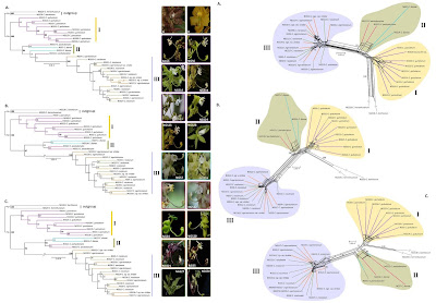
Here's a fused image of the ML trees (their fig. 1) and the corresponding neighbor-nets (their fig. 2):

Not so "phenetic": NGS data neighbor-nets (NNet) show essentially the same than ML trees — the distance matrices reflect putative common origin(s) as much as the ML phylograms. The numbers at branches and edges show bootstrap support under ML and the NNet optimization.

Groups resolved as clades, Group I and III, or grades or clades, Group II (compare A vs. B and C), in the ML trees form simple (relating to one edge-bundle) or more complex (defined by two partly compatible edge-bundles, Group I in A) neighborhoods in the neighbor-net splits graphs. The evolutionary unfolding, we are looking at closely related biological units, was likely not following a simple dichotomizing tree, hence, the ambiguous branch-support (left) and competing edge-support (right) for some of the groups. Furthermore, each part of a genome will be more descriminative for some aspect of the coalescent and less for another, another source of topological ambiguity (ambiguous BS support) and incompatible signal (as seen in and handled by the neighbor-nets). The reconstructions under A, B and C differ in the breadth and gappyness of the included data (all NGS analyses involve data filtering steps): A includes only loci covered for all taxa, B includes all with less than 50% missing data, and C all loci with at least 15% coverage.

PS I contacted the first author, the paper is still under review (four peers), a revision is (about to be) submitted, and, with a bit of luck, we'll see it in print soon.


Example 2: The oaks of the world

The Hipp et al. (note that I am an author) neighbor-net is based on model-based distances. The reason I opted (here) for model-based distance instead of uncorrected p-distances is the depth of our phylogeny: our data cover splits that go back till the Eocene, but many of the species found today are relatively young. The dated tree analyses show substantial shifts in diversification rates. In the diverse lineages today and possibly in the past (see the lines in the following graph), in those with few species (*,#) we may be looking at the left-overs of ancient radiations.

A lineage(s)-through-time plot for the oaks (Hipp et al. 2019, fig. 2). Generic diversification probably started in the Eocene around 50 Ma, and between 10–5 Ma parts (usually a single sublineage) of these long-isolated intrageneric lineages (sections) underwent increased speciation.

The data basis is otherwise similar, SNPs (single-nucleotide polymorphisms) generated using a different NGS method, in our case RAD-tagging (RAD-seq) of c. 450 oak individuals covering the entire range of this common tree genus — the most diverse extra-tropical genus of the Northern Hemisphere. There are differences between GBS and RAD-seq SNP data sets — a rule of thumb is that the latter can provide more signal and SNPs, but the single-loci trees are usually less decisive, which can be a problem for coalescent methods and tests for reticulation and incomplete lineage sorting that require a lot of single-loci (or single-gene) trees (see the paper for a short introduction and discussion, and further references).

We also inferred a ML tree, and my leading co-authors did the other necessary and fancy analyses. Here, I will focus on the essential information needed to interpret the neighbor-net that we show (and why we included it at all).

Our fig. 6. Coloring of main lineages (oak sections) same as in the LTT plot. Bluish, the three sections traditionally included in the white oaks (s.l.); red, red oaks; purple, the golden-cup or 'intermediate' (between white and red) oaks — these three groups (five sections) form subgenus Quercus, which except for the "Roburoids" and one species of sect. Ponticae is restricted to the Americas. Yellow to green, the sections and main clades (in our and earlier ML trees) of the exclusively Eurasian subgenus Cerris.

Like Pérez Escobar et al., we noted a very good fit between the distance-matrix based neighbor-net and the optimised ML tree. Clades with high branch support and intra-clade coherence form distinct clusters, here distinct neighborhoods associated with certain edge bundles (thick colored lines). This tells us that the distance-matrix is representative, it captures the prime-phylogenetic signal that also informs the tree.

The first thing that we can infer from the network is that we have little missing data issues in our data. Distance-based methods are prone to missing data artifacts and RAD-seq data are (inevitably) rather gappy. It is important to keep in mind that neighbor-nets cannot replace tree analysis in the case of NGS data, they are "just" a tool to explore the overall signal in the matrix. If the network has neighborhoods contrasting what can be seen in the tree, this can be an indication that one's data is not sufficiently tree-like at all. But it also can just mean that the data is not sufficient to get a representative distance matrix.

Did you notice the little isolated blue dot (Q. lobata)? This is such a case — it has nothing to do with reticulation between the blue and the yellow edges, it's just that the available data don't produce an equally discriminative distance pattern: according to its pairwise distances, this sample is generally much closer to all other oak individuals included in the matrix in contrast to the other members of its Dumosae clade, which are generally more similar to each other, and to the remainder of the white oaks (s.str., dark blue, and s.l., all bluish).

Close-up on the white oak s.str. neighbor-hood (sect. Quercus) and plot of the preferred dated tree.

In the tree it is hence placed as sister to all other members, and, being closer to the all-ancestor, it triggers a deep Dumusae crown age, c. 10 myr older than the subsequent radiation(s) and as old as the divergence of the rest of the white oaks s.str.

The second observation, which can assist in the interpretation of the ML tree (especially the dated one), is the principal structure (ordering) within each subgenus and section. The neighbor-net is a planar (i.e. 2-dimensional graph), so the taxa will be put in a circular order. The algorithm essentially identifies the closest relative (which is a candidate for a direct sister, like a tree does) and the second-closest relative. Towards the leaves of the Tree of Life, this is usually a cousin, or, in the case of reticulation, the intermixing lineage. Towards the roots, it can reflect the general level of derivation, the distance the (hypothetical all-)ancestor.

Knowing the primary split (between the two subgenera), we can interprete the graph towards the general level of (phylogenetic) derivedness.

The overall least derived groups are placed to the left in each subgenus, and the most derived to the right. The reason is long-branch attraction (LBA) stepping in: the red and green group are the most isolated/unique within their subgenera, and hence they attract each other. This is important to keep in mind when looking at the tree and judge whether (local) LBA may be an issue (parsimony and distance-methods will always get the wrong tree in the Felsenstein Zone, but probabilistics have a 50% chance to escape). In our oak data, we are on the safe side. The red group (sect. Lobatae, the red oaks) are indeed resolved as the first-branching lineage within subgenus Quercus, but within subgenus Cerris it is the yellow group, sect. Cyclobalanopsis. If this would be LBA, Cyclobalanopsis would need to be on the right side, next to the red oaks.

The third obvious pattern is the distinct form of each subgraph: we have neighborhoods with long, slim root trunks and others that look like broad fans.

Long-narrow trunks, i.e. distances show high intra-group coherence and high inter-group distinctness can be expected for long isolated lineages with small (founder) population sizes, eg. lineages that underwent in the past severe or repeated bottleneck situations. Unique genetic signatures will be quickly accumulated (increasing the overall distance to sister lineages), and the extinction ensures only one (or very similar) signature survives (low intragroup diversity until the final radiation).

Fans represent gradual, undisturbed accumulation of diversity over a long period of time, eg. frequent radiation and formation of new species during range and niche expansion – in the absence of stable barriers we get a very broad, rather unstructured fan like the one of the white oaks (s.str.; blue); along a relative narrow (today and likely in the past) geographic east-west corridor (here: the  'Himalayan corridor') a more structured, elongated one as in the case of section Ilex (olive).

Close-up on the sect. Ilex neighborhood, again with the tree plotted. In the tree, we see just sister clades, in the network we see the strong correlation between geography and genetic diversity patterns, indicating a gradual expansion of the lineage towards the west till finally reaching the Mediterranean. Only sophisticated explicit ancestral area analysis can possibly come to a similar result (often without certainty) which is obvious from comparing the tree with the network.

This can go along with higher population sizes and/or more permeable species barriers, both of which will lead to lower intragroup diversity and less tree-compatible signals. Knowing that both section Quercus (white oaks s.str., blue) and Ilex (olive) evolved and started to radiate about the same time, it's obvious from the structure of both fans that the (mostly and originally temperate) white oaks produced always more, but likely less stable species than the mid-latitude (subtropical to temperate) Ilex oaks today spanning an arc from the Mediterranean via the southern flanks of the Himalayas into the mountains of China and the subtropics of Japan.

Networks can be used to understand, interpret and confirm aspects of the (dated) NGS tree.

The much older stem and young crown ages seen in dated trees may be indicative for bottlenecks, too. But since we typically use relaxed clock models, which allow for rate changes and rely on very few fix points (eg. fossil age constraints), we may get (too?) old stem and (much too) young crown ages, especially for poorly sampled groups or unrepresentative data. By looking at the neighbor-net, we can directly see that the relative old crown ages for the lineages with (today) few species fit with their within-lineage and general distinctness.

The deepest splits: the tree mapped on the neighbor-net.

By mapping the tree onto the network, and thus directly comparing the tree to the network, we can see that different evolutionary processes may be considered to explain what we see in the data. It also shows us how much of our tree is (data-wise) trivial and where it could be worth to take a deeper look, eg. apply coalescent networks, generate more data, or recruit additional data. Last, but not least, it's quick to infer and makes pretty figures.

So, try it out with your NGS data, too.

PS. Model-based distances can be inferred with the same program many of us use to infer the ML tree: RAxML. We can hence use the same model assumptions for the neighbor-net that we optimized for the inferring tree and establishing branch support.

A jolly, holly network ... of Christmas carols

Today is Christmas Eve. What could be more befitting for our merry blog than to show a network of Christmas carols?

The perfect result would, of course, be a snowflake-like network. Ideally, approaching what is called a "stellar dendrite snowflake".

Stellar dendrites. (Images from a post
introducing a snowflake book:
The Snowflake.)

The data

I browsed the internet for lyrics of Christmas carols, and then scored their content in the form of a binary matrix.

The "taxon set" includes 45 traditional and (more) modern carols, some of them listed here, along with some others I remembered and sought out (eg. here). A comprehensive list of traditional carols can be found here, but using this would have made the matrix much too large for a post on Christmas Eve. (If you are reading this before Christmas, you might be spending too much time on science.) A rule of thumb is that a matrix should always have at least as many (completely defined) characters as taxa.

The 45 (hohoho!) "characters" include:

• length (short = 0, long = 1), and tone (merry = 0, darkish = 1)
• topics it is about / relates to / mentions — e.g. the birth scene, love, and yuletide (the latter included because as a naturalized Swede, I love the jultiden, fancy julkaffe, and much enjoyed most of my julbord);
• major Christmas figures — Jesus, angels, drummers, elves, Jack Frost, the Grinch, milking maids, monsters, Santa Claus, shepherds, snowmen, the Wise Men from the Orient;
• mentioned animals, such as reindeer, and plants, including the Christmas tree (traditionally a Tannenbaum – fir tree), and (very important for Anglosaxons who don't kiss each other whenever they meet, like we do in France) the mistletoe
• last but not least, Christmas related objects — non-living things such as bells, Christmas food, harps, sleighs, snow, stars, and presents.

The network

The result is not a perfect stellar dendrite, but it is close enough.

A Neighbor-net of Christmas carols. Stippled terminal edges are reduced by factor 2.

It has quite a nice circular sorting of the carols, each related in some way to the ones next to it. The only oddly placed one is "Twelve Days of Christmas", which is a very peculiar one (and my English, favorite), along with the rather content-free "We wish You a Merry Christmas".

Finally, as a Christmas treat, the "great voices of the British public" singing (and reflecting on) my favorite carol: a Creature Comforts Christmas special.

A merry Christmas to everyone!

And please try out some networks during the coming year.

Please stop using cladograms!

I really like the journal PeerJ, not only because it is open access and publishes the peer review process, but also because it's one of the few that adhere to strict policies when it comes to data documentation. In my last (on my own) 2-piece post (part 1, part 2), I showed what networks could have offered for historical and more recent studies in Cladistics, the journal of the Willi Hennig Society. In this one, I'll illustrate why paleontology in general needs to stop using cladograms.

An example

In a recent article, Atterholt et al. (PeerJ 6: e5910, 2018) describe and discuss "the most complete enantiornithine from North America and a phylogenetic analysis of the Avisauridae". I'm not a paleozoologist and "stuff of legend", but their first 17 figures seem to make a good point about the beauty of the fossil and its relevance; and it is interesting to read about it. This makes me envy paleozoologists a bit — the reason I exchanged chemistry for paleontology was my childhood love for the thunder lizards; I specialized in zoology not botany for graduate biology courses, and I fell in love with social insects, especially bees; but then more general circumstances pushed me into plant phylogenetics.

The result of Atterholt et al.'s phylogenetic analysis is presented in their figure 18, as shown here.

Figure 18 of Atterholt et al. (2018): "A cladogram depicting the hypothetical phylogenetic position of Mirarce eatoni." [the beautiful fossil is highlighted in bold font]

This looks very familiar — graphs like this can be seen in many paleontological studies, not only those in Cladistics. However, this is a phylogeneticist's "nightmare" (but a cladist's "dream").

First, phylogenetic trees, especially those that were weighted post-analysis several times to get a more or less resolved tree, should be depicted as phylograms — trees with branch lengths. Phylogenetic hypotheses are not only about clades, and what is sister to what, but about the amount of (inferred) evolutionary change between the hypothetical ancestors, the internal nodes, and their descendants, the labelled tips. For example, we may want to know how long is the root of the clade (Avisauridae, Avisaurus s.l.) comprising the focus taxon compared to the lengths of the terminal branches within the clade. Prominent roots and short terminals are a good sign for monophyly (inclusive common origin), or at least a fossil well placed, whereas short roots and long terminals are not.

The above tree as phylogram (using PAUP*'s AccTran optimization). The beauty of cladistic classification is that the new specimen could have just been described as another species of Avisaurus (but read the author's discussion).

In this example, we seem to be on the safe side, although one may question the general taxonomic concept for extinct birds. Are the differences enough to erect a new genus for every specimen? This is hard to decide based on this matrix.

Second, a tree without branch support is just a naked line graph, telling us nothing about the quality (strengths and weaknesses) of the backing data. Neontologists are not allowed to publish naked trees. In molecular phylogenetics, we are not uncommonly asked by reviewers to drop all branches (internodes) below an arbitrary threshold: a bootstrap (BS) support value < 70 and posterior probability (PP) < 0.95. In palaentology, it has become widely accepted to not show support values at all. The reason is simple: the branch support is always low, because of data gaps and homoplasy. This is a problem the authors are well aware of:

The modified matrix consists of 43 taxa (26 enantiornithines, 10 ornithuromorphs) scored across 252 morphological characters [the provided matrix lists 253], which we analyzed using TNT (Goloboff, Farris & Nixon, 2008a). Early avian evolution is extremely homoplastic (O’Connor, Chiappe & Bell, 2011; Xu, 2018) thus we utilized implied weighting (without implied weights Pygostylia was resolved as a polytomy due to the placement of Mystiornis) (Goloboff et al., 2008b); we explored k values from one to 25 (see Supplemental Information) and found that the tree stabilized at k values higher than 12. In the presented analysis we conducted a heuristic search using tree-bisection reconnection retaining the single shortest tree from every 1,000 replications with a k-value of 13. This produced six most parsimonious trees with a score of 25.1. These trees differed only in the relative placement of five enantiornithines closely related to the Avisauridae, forming a polytomy with this clade in the strict consensus tree (Consistency Index = 0.453; Retention Index = 0.650; Fig. 18).

I've seen much worse CI and RI values in the paleophylogenetic literature (some of them are plotted in this post). For a phylogenetic inference, homoplasy equals internally incompatible signals — many characters show different, partly or fully conflicting, taxon bipartitions; or, in other words, they prefer different trees. The signal in the matrix is thus not tree-like — it doesn't fit a single tree. That's why we have to choose one using TNT's iterated reweighting procedures. (Note: an alternative "phenetic" Neighbor-joining tree has a computation time < 1s, and produces the same tree for the Ornithumorpha and the root-proximal, 'basal' part of the tree, except that Jeholornis is moved two nodes up; but it shuffles a lot in the Longirostravis–Avisauridae clade.)

Another point is that the more homoplasy we have, then the higher must have been the rate of change (here: visible anatomical mutation). The higher the rate of change, the higher the statistical inconsistency of parsimony.

In short, paleontologists (Atterholt et al. just follow the standard in paleophylogenetic publications) use data with tree-unlike signal to infer trees (see also David's last post on illogicality in phylogenetics) under a possibly invalid optimality criterion, which are then used to downweight characters (eliminate noise due to homoplasy) to infer less noisy, "better" trees.

The basic signal

We can't change the data, but we can explore and show its signal. And the basic signal from the unfiltered matrix is best visualized using a Neighbor-net splits graph.

Neighbor-net based on mean pairwise taxon distances. Thick edges correspond to branches in the published tree.

Some differentiation patterns that explain the clades in the tree can be traced, but it becomes difficult in the group that is of most interest: the (inferred) clade(s) comprising the newly described fossil. In the Neighbor-net this is placed close to another member of the Avisauridae, but not all. The matrix is not optimal for the task at hand.

The data properties

The matrix is a multistate matrix with up to six states in the definition line (although only five are used, as state "5" is not present). The taxa have variable gappyness (i.e. the proportion of completely undetermined cells), between 2% (extant birds: Anas and Gallus) and 94% (Intiornis, an Avisauridae) — the median is 56%, and the average close to it (54%). The "hypothetically" placed fossil Mirarce eatoni (in the matrix it is under its old designation: "Kaiparowits") lacks a bit more of the scored characters (61%). That may strike one as a lot, but note that the matrix has 253 characters! However, we may well ask: if I want to place a fossil for which I can score 99 characters, why bother to include another ~150 that tell me nothing about its affinity? (Note: paleobotanists struggle hard even to get such numbers, we usually have at best 50 characters.)

Its closest putative relatives, the Avisaurus s.l., lack 90% of the characters; leaving us with max. 25 characters supporting the relevant clade (assuming that the 10% are all found in Mirarce as well). Coverage is not much better in the next-closest relatives (phylogenetically speaking).

Data coverage in the phylogenetic neighborhood of Mirarce eatoni

The missing data percentage may have mislead the Neighbor-net a bit, because we will have fed it with unrepresentative or highly ambiguous pairwise distances. In the the network, the focus fossil comes close to Neuquenornis, the only other Avisauridae with some data coverage. Looking at the heat map below, we see that missing data is indeed a problem in this matrix — we have zero distances between several pairs that show different distances to the better-covered taxa.

The distance matrix drawn as a heat map: green = similar, red = dissimilar (values range between 0 and 0.8). Red arrows: taxa with too many (and ambiguous) zero pairwise distances.

The closest relative of Mirarce is, indeed, Avisaurus/Gettya gloriae, but the latter has zero distances to various other poorly covered taxa from the phylogenetic neighborhood, in contrast to the much better-covered Mirarce. Neighbor-nets are very good at getting the obvious out of a morphological matrix, but they don't perform miracles. However, why should we include poorly known taxa at all during phylogenetic inference? Wouldn't it be better to infer a backbone tree (or network showing the alternative hypotheses) based on a less gappy matrix, and then find the optimal position of the poorly known taxa within that tree (network)?

Estimating the actual character support

Some characters cover just 10–20% of the taxa, whereas others are scored for most of them — more than half of the characters are missing for more than half of the taxa. Using TNT's iterative weight-to-fit option means that we infer a tree, ideally one fitting the well-covered data (taxon- and character-wise), and then downweight all conflicting characters elsewhere to fit this tree. We then end up with a tree where we have no idea about actual character support. Since the matrix is a Swiss cheese, we only can re-affirm the first-inferred tree.

Let's check the raw character support, using non-parametric bootstrapping and maximum likelihood as the optimality criterion (corrected for ascertainment bias, as implemented in RAxML).

ML-BS Consensus Network (using Lewis' 2-parameter Mk+G model). Edge lengths are proportional to the BS support values of taxon bipartitions (= phylogenetic splits, internodes, branches in phylogenetic trees). Only splits are shown that occurred in at least 10% of 900 BS pseudoreplicates (number of necessary BS replicates determined by the Extended Majority Rule Bootstrap criterion), trivial splits collapsed. Thick edges correspond with branches in Atterholt et al.'s iterative parsimony tree; coloring as before.

The ML bootstrap Consensus Network bears not a few similarities to the distance-based Neighbor-net. The characters do not support the Avisauridae subtree, as depicted in the published TNT tree, but there are faint signals associating some of them to each other, despite the missing data. Keep in mind: a BS support of 20 for one alternative and < 10 for all others means (ideally) one fifth of the characters support the split, and the rest have no (coherent) information. Some sister pairs have quite high support (for this kind of data set), and Gettya gloriae is resolved as sister of Mirarce (unambiguously, with a BS support = 67). But, the matrix hardly has the capacity to resolve deeper relationships within the group of interest, the Enantiornithes — the polytomy with the next relatives seen in the tree and the corresponding clade dissolve. This confirms what we saw in the Neighbor-Net (despite missing data distortion).

The matrix and the tree show something that could have been deduced directly from the distance matrix: the poorly known Gettya (Avisaurus) gloriae is (literally) the closest relative of the enigmatic new genus / species Mirarce (morphological distance of 0.08 compared to 0.1–0.64 for all other taxa). But is this overall similarity enough to conclude Avisaurus, Gettya and Mirarce are a monophyletic group within the Avisauridae?

What the authors (and all paleontologists doing phylogenetics) should have done

(I would have skipped all trees, naturally, but peer reviewers and most readers probably need to see them.)

• Trimmed the matrix to include only those characters preserved in the fossil of interest, in order to minimize missing data artefacts during inference.
• Shown the Neighbor-net to visualize the primary signal situation, including and excluding poorly covered taxa. From the Neighbor-net it is already obvious that the fossil is an Enantiornithes, so any subsequent optimization / inference could have focussed on this group alone.
• Then inferred a backbone tree excluding poorly covered taxa, and shown the resulting phylogram. In case one needs to test the Enantiornithes root (the Neighbor-net gives us two alternatives for the Enantiornithes root: Pengornis + Eopengornis or Protopteryx + Iberomesornis), there is no point in including the poorly covered Enantiornithes or the worst-covered taxa outside this clade.
• Then optimized the position of the poorly covered taxa in the backbone tree. I recommend using RAxML's evolutionary placement algorithm (EPA) for this, but you can also do this in a parsimony framework if you wish. (EPA can also be used to test outgroup roots: here, one would search the branch at which all non-Enantiornithes fit best.)
• Shown the resulting phylogram including all taxa — that is, read in the topology to the analysis, and then re-optimize branch lengths.
• Shown a Support Consensus Network to illustrate the support for the branches in the preferred tree and their competing alternatives. (There may be one or more, as there are many options to estimate branch support.) How sure can we be about relationships within the Avisauridae and their relationships to other Enantiornithes?

---

Postscriptum. For those who are curious about how the ML tree would look like, here it is:

I have no idea about birds, but from a methodological point of view this is an equally (if not more, because unforced) valid hypothesis for the data set. And demonstrating its limitations: note the relatively long branches with very low support making up the backbone of the Enantiornithes clade. This is typical for matrices lacking coherent discriminatory signal and/or struggling with internal conflict.

More heretic bits: networks for (more) recent matrices published in Cladistics

This is Part 2 of a 2-part blog series. Part 1 covered some history, while this post has three (more) recently published matrices, and the take-home message.

Jumping forward in time, welcome to the 21st century

In Part 1, I showed several networks generated based on some early phylogenetic matrices published in the first volumes of the journal Cladistics. In this post, we will look at the most recent data matrices and trees uploaded to TreeBASE, covering the past seven years.

Nearly a generation later, and facing the "molecular revolution", some researchers (fortunately) still compile morphological matrices. This is an often overlooked but important work: genes and genomes can be sequenced by machines, and the only thing we need to do is to feed these machine-generated data into other powerful machines (and programs) to get a phylogenetic tree, or network. But no software and computer cluster can (so far) study anatomy, and generate a morphological matrix. The latter is paramount when we want to put fossils, usually devoid of DNA, in a (molecular) phylogenetic context. We need to do this when we aim to reconstruct histories in space and time.

Nevertheless, we can't ignore the fact that these important data are (still) far from tree-like. What holds for the matrices of the 80's (see the end of Part 1), still applies now.

So, let's have a look at the three most recent data sets (one morphological, two molecular) published in Cladistics that have their data matrix in TreeBASE.

The morphological dataset

Beutel et al. (2011; submission S11976) provided a "robust phylogeny of ... Holometabola", and note in their abstract: "Our results show little congruence with studies based on rRNA, but confirm most clades retrieved in a recent study based on nuclear genes."

Without having read the study, I can guess which clades (likely used here as a synonym for monophyletic group; but see David's post on Hennig and Cladistics) were confirmed. The data matrix contains: 356 multistate, with up to six states, characters scored and annotated for 34 taxa, including polymorphisms and some gaps ("–") viz missing data ("?"). Just by looking at the Neighbor-net inferred from this matrix. (Standard tree- or network-inference doesn't differ between gaps and missing data, but some people find it important to distinguish between "not applicable" and "not known" in a matrix.)

Neighbor-net inferred from simple pairwise distances computed based on Beutel et al.'s matrix. Brackets show my ad hoc assessment of candidates for monophyla (here: likely represented by clades in no matter how optimized trees).

How did I postulate the monophyla? By deduction: if two or more OTUs are much more similar to each other than to anything else in the matrix, they likely are part of the same evolutionary lineage, ie. have a common origin (= monophyletic in a pre-Hennigian sense). This, when the matrix well covers the group and morphospace, has a good chance to be inclusive (= monophyletic fide Hennig; for the covered OTUs). This is especially so when there is a good deal of homoplasy — the provided tree has a CI of 0.44 and RC of 0.33: convergences should be more randomly distributed than lineage-specific/-conserved traits. The latter don't need to be (or were, at some point in time) synapomorphies, shared derived unique traits, but could be diagnostic suites of characters that evolved in parallel within a lineage and passed on to all (or most) of the descendants.

The first molecular dataset

Let's look at the signal in the two molecular matrices.

In 2016, Gaspar and Almeida (submission S19167) tested generic circumscriptions in a group of ferns by "assembl[ing] the broadest dataset thus far, from three plastid regions (rbcL, rps4-trnS, trnL-trnF) ... includ[ing] 158 taxa and 178 newly generated sequences". They found: "three subfamilies each corresponding to a highly supported clade across all analyses (maximum parsimony, Bayesian inference, and maximum likelihood)."

The total matrix has 3250 characters, of which 1641 are constant and 1189 are parsimony-informative. This is a quite a lot for such a matrix, and, by itself, rules out parsimony for tree-inference. If half of the nucleotide sites are variable, then the rate of character change was high, and parsimony is statistically only robust, when the rate of change was low. High mutation rates or high level of divergence may also pose problems for distance methods and other optimality criteria, all closely related to parsimony.

The file includes three trees, labelled "vero" (which, in Italian, means "true"), "Fig._1" and "MPT". "Vero" and "Fig._1" come with branch lengths; judging from the values (<< 1), they are probabilistic trees (of some sort); the "MPT" is (as usual) provided as a cladogram without branch-lengths. It may be that the authors had to add the parsimony tree just to fulfill editorial policies, while being convinced "vero" is the much better tree. "Vero" is a fully resolved tree (the ML tree?), while "Fig._1" (Bayesian?) and "MPT" include polytomies.

Using PAUP*'s "describe" function, we learn that the "MPT" is 5101 steps long and has a CI of 0.41 and RC of 0.33. Nucleotide sequence data can be notoriously homoplasious, as we repeat the same four states into infinity and have to deal with an unknown but usually significant amount of back mutations. This adds to the other problems for parsimony:

• transitions are more likely to happen than transversions; and
• in coding gene regions, such as the rbcL, some sites (3^rd codon positions) mutate much faster than others.

Still, parsimony trees are not necessarily wrong. Neither are NJ trees; and there are also datasets where probabilistic methods struggle, eg. when the likelihood surface of the treespace is flat.

So, the first question is: how different are the three trees provided? Rather than having to show three graphs, we can show the (strict) Consensus network of those trees.

A strict consensus network summarizing the topologies of the three trees provided in the TreeBASE submission of

The main difference is between "vero" and the other two — "Fig. 1" and the "MPT" are very similar (and both include polytomies). There are three main scenarios for a Consensus network like this with respect to the high portion of variable sites:

1. "Fig. 1" is a Jukes-Cantor model-based tree,
2. "Fig. 1" is an uncorrected p-distance based tree, or
3. most of the variation is between ingroup (the subtree including all Blechnum) and outgroup (the other subtree).

"Vero" is still quite congruent, so the model used here can't be too much different, either.

What should ring one's alarm bells are, however, the many grade-like / staircase subtrees, which are unusual for a molecular data set. Staircases imply that each subsequent dichotomous speciation event resulted in a single species and a further diversifying lineage: multiple, consistently occurring budding events.

The same graph, with arrows showing grade evolution. Often found in morpho-data-based trees with ancestral, more ancient, and derived (from them), modern forms, but should ring an alarm bell when common in a molecular tree. Major clades (found in all three trees) are labelled for comparison with the next graph.

Let's compare this to the Neighbor-net (usually, I would use model-based distances in such a case, but here we can do with uncorrected p-distances).

A Neighbor-net inferred from uncorrected p-distances based on Gaspar & Almeida's matrix; the major clades are labelled as in the preceding graph. Note the isolated, long-branch blue dots with asterisks, indicating the position of the first diverged species in the large clades G and I. Genuine signal or missing data artefact?

The Neighbor-net shows only a limited number of tree-like portions, but does correspond with the main clades above. Only A and B are dissolved, which are the two first diverging clades in the original trees (preceding graph). Some OTUs are placed close to the centre of the graph, or even along a tree-like portion (purple dots), a behaviour known from actual ancestors: some OTUs apparently have sequences that may be literally ancestral to others. This explains the grade structure seen in the original trees. Others (violet dots) create boxes, which may reflect a genuine ambiguous signal, or just be missing data leading to ambiguous pairwise distances. The latter (missing data artefact) is behind the misplacement of the four OTUs (red dots): missing data can inflate pairwise distances severely. And, like parsimony, distance-based methods are more vulnerable to long-branch(edge)-attraction than probabilistic methods.

Model-based distances may help clean up this a bit, but the networks needed for these kind of data are Support consensus networks (see e.g. Schliep et al., MEE, 2017). The split appearance of the Neighbor-net hints at internal signal conflict and, with respect to the high number of variable sites (note the sometimes extremely long terminal edges), saturation issues. Two major questions would be:

1. How do the different markers (coding gene vs. inter-genic spacers with different levels of diversity; rps4-trnS is typically more divergent than the trnL-trnF spacer) resolve relationships, which clades / topological alternatives receive unanimous support?
2. Does it make a difference to run a fully partitioned (ML) analysis vs. an unpartitioned one vs. one excluding the 3^rd codon position in the gene?

For intra-clade evolutionary pathways, it would be worthwhile to give median networks and suchlike a try, as parsimony methods that can discern ancestor-descendant relationships.

The second molecular dataset

The most recent data are from Kuo et al. (2017; submission S20277), who inferred a "robust ... phylogeny" (see Part 1, Jamieson et al. 1987, and Beutel et al., above) for a group of ferns, focusing on the taxonomy of a single genus, Deparia, that now includes five traditionally recognized genera. In the abstract it says: "... seven major clades were identified, and most of them were characterized by inferring synapomorphies using 14 morphological characters".

The matrix includes the molecular characters used to infer the major clades plus two trees, labelled "bestREP1" and "rep9BEST", both with branch lengths. Branch length values indicate that "bestREP1" could be parsimony-optimized (with averaged or weighted branch lengths), while "rep9BEST" is either a ML or Bayesian tree (technically, it could be a distance-based tree, too, but I don't think such "phenetics" are condoned by Cladistics).

Re-calculated, the first tree ("bestREP1") is shorter (3024 steps) than the one of Gaspar & Almeida, reflecting the much lower number of parsimony-informative sites (979). Many of the sites differ only between the focal genus and the outgroups, which is well visible in the Neighbor-net. [For those of you unfamiliar with Neighbor-nets, a parsimony analysis of these data takes hours, or days depending on the software and computer, while the distance matrix and the resultant Neighbor-net is inferred in a blink.]

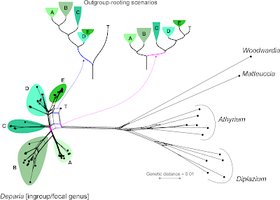
The Neighbor-net based on Kuo et al.'s data. Why do we need to include long-branching, distant outgroups when we just want to bring order in a genus? Because to test monophyly, we need a rooted tree (ambiguous or not, or even biased by branching artefacts).

Let's remove the distant, long-branching outgroups, which (as we can see in the Neighbor-net) at best provide ambiguous signal for rooting the ingroup — at worst, they trigger ingroup-outgroup branching artefacts. What could a Neighbour-net have contributed regarding taxonomy and the seven major monophyletic intrageneric groups ("clades")? Pretty much everything needed for the paper, I guess (judging from the abstract).

Same data as above, but outgroups removed. The structure of this Neighbour-net allows to identify seven likely candidates for monophyla ("1"–"7"), with "1" and "2" being obvious sister lineages. Colours refer to the clusters ("A"–"E") annotated above.

On a side note: by removing the long-branching, distant outgroups, taxon "T" is resolved as a probable member of the putative monophyletic group "5" (= "E" in the full graph with outgroups, and surely a high-supported subtree in any ingroup-only reconstruction, method-independent). Placing the root between "T" and the rest of the genus implies that "5" is a paraphyletic group comprising species that haven't evolved and diversified at all (ie. are genetically primitive), in stark contrast to the other main intra-generic lineages. This is not impossible, but quite unlikely. More likely is the second scenario (primary split between "1"–"3" and "4"–"7"). Having "4" as sister to the rest could be an alternative, too.

This is where Hennig's logic could be of help: find and tabulate putative synapomorphies to argue for a set and root that makes the most sense regarding morphological evolution and molecular differentiation.

The take-home message(s)

We have argued before that it is in the ultimate interest of science and scientists to give access to phylogenetic data. No matter where one stands regarding phylogenetic philosophy, we should publish our data, so that people can do analyses of their own. Discussion should be based on results, not philosophies.

When you deal with morphological data, you should never be content with inferring a single tree (parsimony or other). You have to use networks.

The Neighbor-net was born as late as 2002 (Bryant & Moulton, 2002, in: Guigó R, and Gusfield D, eds, Algorithms in Bioinformatics, Second International Workshop, WABI, p. 375–391; paywalled) and made known to biologists in 2004 (same authors, same title, in Mol. Biol. Evol. 21:255–265), so that authors before this time did not have access to its benefits. Similarly, Consensus networks arrived around about the same time (Holland & Moulton 2003, in: Benson G, and Page R, eds, Algorithms in Bioinformatics: Third International Workshop, WABI, p. 165–176). However, the Genealogical World of Phylogenetic Networks has been here for six years now (first post February 2012). So there is now no excuse for publishing a cladogram without having explored the tree-likeness of your matrix' signal!

Neighbor-nets like the ones I showed in this 2-piece post (or can be found in many of our other posts) are a quick and essential tool to explore the basic signal in your matrix:

• How tree-like is it?
• Where are the potential conflicts, obscurities?
• What are the principal evolutionary alternatives (competing topologies)?
• What is well supported (especially regarding taxonomy and the question of monophyly)?

Even if you don't use it in your paper, the network will tell you what you are dealing with when you start inferring trees.

The second essential tool is the much under-used Support consensus network, not shown in this post but in plenty of our other posts (and many papers I co-authored; for a comprehensive collection of network-related literature see Who's who in phylogenetic networks by Philippe Gambette). Support consensus networks estimate and visualize the robustness of the signal for competing topological (tree) alternatives.

Consensus networks should also be obligatory for those molecular data,where even probabilistic methods fail to find a single fully resolved, highly supported tree.

If the editors of Cladistics are really dedicated to parsimony, they should not still insist only on a parsimony tree (often provided as cladogram), but also parsimony-based networks as well:

• strict Consensus networks to summarize the MPT samples instead of the standard strict Consensus cladograms;
• bootstrap Support consensus networks showing the signal strength and support for alternative trees/competing clades (TNT has many bootstrapping options to play around with); and
• Median networks and such-like for datasets with few mutations, and low levels of expected homoplasy.

This is what the 2016 #parsimonygate uproar (see Part 1) should have been about (12 years after Neighbor-nets, and 11 years after Consensus networks). Not the prioritizing of parsimony, but the naivety or ignorance towards pitfalls of (parsimony or other) trees inferred from data not providing tree-like signal or riddled by internal conflict.
This is a problem not limited to Cladistics, but found, to my modest experience in professional science (c. 20 years), in many other journals as well (e.g. Bot. J. Linn. Soc., Taxon, Mol. Phyl. Evol., J. Biogeogr., Syst. Biol., Nature, Science).

Hence, here are my suggestions for future conference buttons, instead of those shown in Part 1.

No Cladograms!

Use Neighbour-nets!

Support Consensus Networks as obligatory!

Further reading for those who mistrust trees or become network-curious in general

• In this blog, under the label "EDA" you will find all sorts of data-display / data-explaining networks, biological and non-biological ones; and the labels "neighbor-net" and "consensus networks" will point you to posts using these networks.
• For problem trees – ancestor-descendant relationships, see this recent post and the posts linked there. In this context, don't miss our posts on median networks.
• The label "treelikeness" brings you to posts questioning trees inferred from non-treelike data.
• The labels "cladistics" and "philosophy" include also more conceptual posts in our strife for less tree-thinking and more network-thinking.
• The labels "phylo-networks" and "branch support" collect similar posts on my science-and-other-stuff blog Res.I.P.