Stacking networks based on sign language manual alphabets

This post is the first of a mini-series on sign language manual alphabets. While the evolution of spoken languages has been studied intensively using phylogenetic methods, sign languages have not, as yet.

In this post we will first introduce our readers to a set of stacked networks, and how it assists in establishing ancestor-descendant relationships in a pretty straightforward (but not trivial) case: the evolution of manual alphabets in sign languages. In the next post, I will demonstrate the use of networks for character mapping and putting forward hypothesis about ancestor-descendant relationships.

In 2004, Spencer et al. (Two papers you may want to read...) showed that Neighbor-nets outperform tree inferences when it comes to explicit ancestor-descendant relationships. The data set they used was quite particular: copies of written text. Here, scribes copy a text, and then other scribes, some of them ignorant of the language of the text they are copying, copy the copies. In the paper, the sequence of copies was recorded (the 'true tree'), and then the various texts were transferred into phylogenetic matrices, in order to infer trees and networks, and then this result was compared to the 'true tree'. The best fit of the data to the truth was the Neighbor-net.

This is a compelling conclusion, because, as a planar network and in contrast to median networks, Neighbor-nets don't explicitly place taxa in ancestor-descendant relationships. However, we have shown for many cases here at the Genealogical World of Phylogenetic Networks how ancestors are often placed with respect to their descendants: they are often closer to the center of the graph, or the root when known, and thus they bridge the center or sister lineages and their descendants. We can thus see why Neighbor-nets might be useful in practice.

In this context, the evolution of sign language manual alphabets, ie. the hand-shapes used to represent letters of a written alphabet, should be relatively easy to reconstruct. Once an alphabet is established in a sign language school / community, the ancestor, it will be passed on to other "generations" within the community and other schools / communities, the descendants. However, this is not necessarily a dichotomous process, as depicted in the first figure.

A scheme depicting how manual alphabets may evolve and disperse.

There are a few complications here: for example, hand-shapes may change in course of being used (the hand-shape evolves); contact may lead to exchange or appropriation of hand-shapes (called "borrowing" in linguistics); and, in some cases, entire alphabets will need to be adapted to a particular use. The latter case occurs when changing from one script (Latin, say) to another (Cyrillic or Arabic) — the first formal school for the deaf was established in Paris, for example. As a teacher, I need to decide: Do I take a hand-shape from the morphologically similar letter, or the phonetically similar one? As a scientist, I need to assess the homologies among such hand-shapes without inflicting systematic bias.

Standardization will wipe out local customs and replace them with a multinational standard. For instance, Country 2 in the scheme above, drops its original B-type manual alphabet (red) for an A-type (blue); and in Country 7 both traditions are fused. Over time, originally distinct sign languages may converge due to geographic proximity, or even just feasibility.

The evolution of spoken languages has been studied intensively using phylogenetic methods, and in particular networks are much more commonly found in the linguistic literature than in the biological one. For sign languages we have made a first step in a recently published pre-print:

Justin M. Power, Guido W. Grimm, and Johann-Mattis List (2019) Evolutionary dynamics in the dispersal of sign languages. Humanities Commons. http://dx.doi.org/10.17613/0smt-j414

What excites me about our study is that it combines historical manual alphabets (going back to 1593), which are potential ancestors, with a set of modern-day alphabets, which are their likely descendants. The data set is thus an evolutionary paleontologist's dream (and, possibly, a cladist's nightmare, if we expect a simple tree-like set of relationships rather than a network). As a scientist, I simple love to boldly go where no-one has gone before.

The next figure shows the all-inclusive network from our paper, but focusing on the age of the manual alphabets.

For more linguistic details see the pre-print.
* Historical version(s) of these lineages are not included in our data set

Obviously, there has been quite a lot of evolutionary changes, as well as standardization, going on, although some parts, like the Swedish SL (sign language), have stuck to its unique original. Historical and contemporary Spanish / Catalan are still most similar to the oldest manual alphabets that Justin dug out for our study. On the other hand, the contemporary Norwegian SL is placed far apart from his historical counterparts, and lacks any obvious affinity. Austrian, Danish, and German look back on a long and diverse history, the green "Austrian-origin Group", but the contemporaries have been homogenized by standardization (note the closeness to the International Sign manual alphabet). If we use an analogy with common biological and biogeographical processes (such as range expansion, competition, extinction, etc), then the Austrian-origin Group only survived in a remote island population, where we still find a sort of living fossil, the Icelandic SL.

In contrast to biological data, the old, putatively ancestral, manual alphabets are not closer to the graph's center, or the oldest manual alphabets in our data set. The reason for this seems to lie in the data itself and how manual alphabets evolve, and this will be the topic of the next post(s).

Still, we can isolate some evolutionary pathways, especially when we make time-wise taxon-filtered networks and stack them (see this introduction to stacking and this application using Osmundaceae, a data set including an even larger ratio of fossil taxa to modern taxa).

Fig. 4 from Power et al. Coloring same as above: pink – Spanish; turquoise – French-origin; green – Austrian-origin; orange – Polish; red – Russian; light blue – Swedish Group. The English-origin and Afghan-Jordanian groups are not included, since not represented by historical manual alphabets in our data set

Each of the three networks includes manual alphabets from a certain time period, starting with pre-1840 at the bottom, historical 19th-/20th-century manual alphabets in the middle, and post-1950 manual alphabets in the top network. The dotted links between the networks connect manual alphabets that are included in two of the networks.

Even from these graphs alone, we can say a lot about how ancestors (original manual alphabets in a country) relate to descendants (later and contemporary manual alphabets) and their evolutionary pathways. Here are some examples.

Shortly after the time when the first schools for the deaf were established in continental Europe (late 18th, early 19th centuries), manual alphabets showed quite a diversity, and were very different from their potential Spanish sources, such as Yebra 1593 and Bonet 1620, with the French and Austrian teachers and communities going different ways. The oldest Cyrillic alphabet, Russian 1835, is more closely related to (ancient) Austrian than it is to (ancient) French.

The Swedish manual alphabet of 1866 is a fresh invention. Some hand-shapes may have been borrowed from one or another alphabet in use on the continent, but, as we will see in the next post of the series, includes genuinely new forms.

The French tradition was dispersed into the new World (American SL appears to be a direct derivation from the French, while the Brazilian SL is an adaptation) but remained a relatively homogeneous group. On the other hand, the Austrian-origin languages diversified, in particular within the Danish influence zone. Politically, the Danish king ceded Norway to Sweden in the Treaty of Kiel 1814 (note the distance between Norwegian and Danish languages in the late 19th century), while Iceland was a Danish dependency until 1918, when the Danish-Icelandic Act of Union was signed. Furthermore, the German manual alphabets subsequently diverged from the Austrian source.

The Polish manual alphabet, originally an adaptation of the Austrian-Danish manual alphabets (see the graph in the middle), became closer to the Russian group, with the Latvian sign language taking up an intermediate position. The Cyrillic alphabets evolved further away, too (top graph).

In the following post(s) of this miniseries, we will explain what we learned from simple character mapping on the time-taxon-filtered networks, and how to score manual alphabets in the first place.


Follow-up posts in this miniseries

• Character cliques and networks: mapping haplotypes of manual alphabets – how we explored the principal signals in our matrix

More heretic bits: networks for (more) recent matrices published in Cladistics

This is Part 2 of a 2-part blog series. Part 1 covered some history, while this post has three (more) recently published matrices, and the take-home message.

Jumping forward in time, welcome to the 21st century

In Part 1, I showed several networks generated based on some early phylogenetic matrices published in the first volumes of the journal Cladistics. In this post, we will look at the most recent data matrices and trees uploaded to TreeBASE, covering the past seven years.

Nearly a generation later, and facing the "molecular revolution", some researchers (fortunately) still compile morphological matrices. This is an often overlooked but important work: genes and genomes can be sequenced by machines, and the only thing we need to do is to feed these machine-generated data into other powerful machines (and programs) to get a phylogenetic tree, or network. But no software and computer cluster can (so far) study anatomy, and generate a morphological matrix. The latter is paramount when we want to put fossils, usually devoid of DNA, in a (molecular) phylogenetic context. We need to do this when we aim to reconstruct histories in space and time.

Nevertheless, we can't ignore the fact that these important data are (still) far from tree-like. What holds for the matrices of the 80's (see the end of Part 1), still applies now.

So, let's have a look at the three most recent data sets (one morphological, two molecular) published in Cladistics that have their data matrix in TreeBASE.

The morphological dataset

Beutel et al. (2011; submission S11976) provided a "robust phylogeny of ... Holometabola", and note in their abstract: "Our results show little congruence with studies based on rRNA, but confirm most clades retrieved in a recent study based on nuclear genes."

Without having read the study, I can guess which clades (likely used here as a synonym for monophyletic group; but see David's post on Hennig and Cladistics) were confirmed. The data matrix contains: 356 multistate, with up to six states, characters scored and annotated for 34 taxa, including polymorphisms and some gaps ("–") viz missing data ("?"). Just by looking at the Neighbor-net inferred from this matrix. (Standard tree- or network-inference doesn't differ between gaps and missing data, but some people find it important to distinguish between "not applicable" and "not known" in a matrix.)

Neighbor-net inferred from simple pairwise distances computed based on Beutel et al.'s matrix. Brackets show my ad hoc assessment of candidates for monophyla (here: likely represented by clades in no matter how optimized trees).

How did I postulate the monophyla? By deduction: if two or more OTUs are much more similar to each other than to anything else in the matrix, they likely are part of the same evolutionary lineage, ie. have a common origin (= monophyletic in a pre-Hennigian sense). This, when the matrix well covers the group and morphospace, has a good chance to be inclusive (= monophyletic fide Hennig; for the covered OTUs). This is especially so when there is a good deal of homoplasy — the provided tree has a CI of 0.44 and RC of 0.33: convergences should be more randomly distributed than lineage-specific/-conserved traits. The latter don't need to be (or were, at some point in time) synapomorphies, shared derived unique traits, but could be diagnostic suites of characters that evolved in parallel within a lineage and passed on to all (or most) of the descendants.

The first molecular dataset

Let's look at the signal in the two molecular matrices.

In 2016, Gaspar and Almeida (submission S19167) tested generic circumscriptions in a group of ferns by "assembl[ing] the broadest dataset thus far, from three plastid regions (rbcL, rps4-trnS, trnL-trnF) ... includ[ing] 158 taxa and 178 newly generated sequences". They found: "three subfamilies each corresponding to a highly supported clade across all analyses (maximum parsimony, Bayesian inference, and maximum likelihood)."

The total matrix has 3250 characters, of which 1641 are constant and 1189 are parsimony-informative. This is a quite a lot for such a matrix, and, by itself, rules out parsimony for tree-inference. If half of the nucleotide sites are variable, then the rate of character change was high, and parsimony is statistically only robust, when the rate of change was low. High mutation rates or high level of divergence may also pose problems for distance methods and other optimality criteria, all closely related to parsimony.

The file includes three trees, labelled "vero" (which, in Italian, means "true"), "Fig._1" and "MPT". "Vero" and "Fig._1" come with branch lengths; judging from the values (<< 1), they are probabilistic trees (of some sort); the "MPT" is (as usual) provided as a cladogram without branch-lengths. It may be that the authors had to add the parsimony tree just to fulfill editorial policies, while being convinced "vero" is the much better tree. "Vero" is a fully resolved tree (the ML tree?), while "Fig._1" (Bayesian?) and "MPT" include polytomies.

Using PAUP*'s "describe" function, we learn that the "MPT" is 5101 steps long and has a CI of 0.41 and RC of 0.33. Nucleotide sequence data can be notoriously homoplasious, as we repeat the same four states into infinity and have to deal with an unknown but usually significant amount of back mutations. This adds to the other problems for parsimony:

• transitions are more likely to happen than transversions; and
• in coding gene regions, such as the rbcL, some sites (3^rd codon positions) mutate much faster than others.

Still, parsimony trees are not necessarily wrong. Neither are NJ trees; and there are also datasets where probabilistic methods struggle, eg. when the likelihood surface of the treespace is flat.

So, the first question is: how different are the three trees provided? Rather than having to show three graphs, we can show the (strict) Consensus network of those trees.

A strict consensus network summarizing the topologies of the three trees provided in the TreeBASE submission of

The main difference is between "vero" and the other two — "Fig. 1" and the "MPT" are very similar (and both include polytomies). There are three main scenarios for a Consensus network like this with respect to the high portion of variable sites:

1. "Fig. 1" is a Jukes-Cantor model-based tree,
2. "Fig. 1" is an uncorrected p-distance based tree, or
3. most of the variation is between ingroup (the subtree including all Blechnum) and outgroup (the other subtree).

"Vero" is still quite congruent, so the model used here can't be too much different, either.

What should ring one's alarm bells are, however, the many grade-like / staircase subtrees, which are unusual for a molecular data set. Staircases imply that each subsequent dichotomous speciation event resulted in a single species and a further diversifying lineage: multiple, consistently occurring budding events.

The same graph, with arrows showing grade evolution. Often found in morpho-data-based trees with ancestral, more ancient, and derived (from them), modern forms, but should ring an alarm bell when common in a molecular tree. Major clades (found in all three trees) are labelled for comparison with the next graph.

Let's compare this to the Neighbor-net (usually, I would use model-based distances in such a case, but here we can do with uncorrected p-distances).

A Neighbor-net inferred from uncorrected p-distances based on Gaspar & Almeida's matrix; the major clades are labelled as in the preceding graph. Note the isolated, long-branch blue dots with asterisks, indicating the position of the first diverged species in the large clades G and I. Genuine signal or missing data artefact?

The Neighbor-net shows only a limited number of tree-like portions, but does correspond with the main clades above. Only A and B are dissolved, which are the two first diverging clades in the original trees (preceding graph). Some OTUs are placed close to the centre of the graph, or even along a tree-like portion (purple dots), a behaviour known from actual ancestors: some OTUs apparently have sequences that may be literally ancestral to others. This explains the grade structure seen in the original trees. Others (violet dots) create boxes, which may reflect a genuine ambiguous signal, or just be missing data leading to ambiguous pairwise distances. The latter (missing data artefact) is behind the misplacement of the four OTUs (red dots): missing data can inflate pairwise distances severely. And, like parsimony, distance-based methods are more vulnerable to long-branch(edge)-attraction than probabilistic methods.

Model-based distances may help clean up this a bit, but the networks needed for these kind of data are Support consensus networks (see e.g. Schliep et al., MEE, 2017). The split appearance of the Neighbor-net hints at internal signal conflict and, with respect to the high number of variable sites (note the sometimes extremely long terminal edges), saturation issues. Two major questions would be:

1. How do the different markers (coding gene vs. inter-genic spacers with different levels of diversity; rps4-trnS is typically more divergent than the trnL-trnF spacer) resolve relationships, which clades / topological alternatives receive unanimous support?
2. Does it make a difference to run a fully partitioned (ML) analysis vs. an unpartitioned one vs. one excluding the 3^rd codon position in the gene?

For intra-clade evolutionary pathways, it would be worthwhile to give median networks and suchlike a try, as parsimony methods that can discern ancestor-descendant relationships.

The second molecular dataset

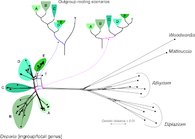
The most recent data are from Kuo et al. (2017; submission S20277), who inferred a "robust ... phylogeny" (see Part 1, Jamieson et al. 1987, and Beutel et al., above) for a group of ferns, focusing on the taxonomy of a single genus, Deparia, that now includes five traditionally recognized genera. In the abstract it says: "... seven major clades were identified, and most of them were characterized by inferring synapomorphies using 14 morphological characters".

The matrix includes the molecular characters used to infer the major clades plus two trees, labelled "bestREP1" and "rep9BEST", both with branch lengths. Branch length values indicate that "bestREP1" could be parsimony-optimized (with averaged or weighted branch lengths), while "rep9BEST" is either a ML or Bayesian tree (technically, it could be a distance-based tree, too, but I don't think such "phenetics" are condoned by Cladistics).

Re-calculated, the first tree ("bestREP1") is shorter (3024 steps) than the one of Gaspar & Almeida, reflecting the much lower number of parsimony-informative sites (979). Many of the sites differ only between the focal genus and the outgroups, which is well visible in the Neighbor-net. [For those of you unfamiliar with Neighbor-nets, a parsimony analysis of these data takes hours, or days depending on the software and computer, while the distance matrix and the resultant Neighbor-net is inferred in a blink.]

The Neighbor-net based on Kuo et al.'s data. Why do we need to include long-branching, distant outgroups when we just want to bring order in a genus? Because to test monophyly, we need a rooted tree (ambiguous or not, or even biased by branching artefacts).

Let's remove the distant, long-branching outgroups, which (as we can see in the Neighbor-net) at best provide ambiguous signal for rooting the ingroup — at worst, they trigger ingroup-outgroup branching artefacts. What could a Neighbour-net have contributed regarding taxonomy and the seven major monophyletic intrageneric groups ("clades")? Pretty much everything needed for the paper, I guess (judging from the abstract).

Same data as above, but outgroups removed. The structure of this Neighbour-net allows to identify seven likely candidates for monophyla ("1"–"7"), with "1" and "2" being obvious sister lineages. Colours refer to the clusters ("A"–"E") annotated above.

On a side note: by removing the long-branching, distant outgroups, taxon "T" is resolved as a probable member of the putative monophyletic group "5" (= "E" in the full graph with outgroups, and surely a high-supported subtree in any ingroup-only reconstruction, method-independent). Placing the root between "T" and the rest of the genus implies that "5" is a paraphyletic group comprising species that haven't evolved and diversified at all (ie. are genetically primitive), in stark contrast to the other main intra-generic lineages. This is not impossible, but quite unlikely. More likely is the second scenario (primary split between "1"–"3" and "4"–"7"). Having "4" as sister to the rest could be an alternative, too.

This is where Hennig's logic could be of help: find and tabulate putative synapomorphies to argue for a set and root that makes the most sense regarding morphological evolution and molecular differentiation.

The take-home message(s)

We have argued before that it is in the ultimate interest of science and scientists to give access to phylogenetic data. No matter where one stands regarding phylogenetic philosophy, we should publish our data, so that people can do analyses of their own. Discussion should be based on results, not philosophies.

When you deal with morphological data, you should never be content with inferring a single tree (parsimony or other). You have to use networks.

The Neighbor-net was born as late as 2002 (Bryant & Moulton, 2002, in: Guigó R, and Gusfield D, eds, Algorithms in Bioinformatics, Second International Workshop, WABI, p. 375–391; paywalled) and made known to biologists in 2004 (same authors, same title, in Mol. Biol. Evol. 21:255–265), so that authors before this time did not have access to its benefits. Similarly, Consensus networks arrived around about the same time (Holland & Moulton 2003, in: Benson G, and Page R, eds, Algorithms in Bioinformatics: Third International Workshop, WABI, p. 165–176). However, the Genealogical World of Phylogenetic Networks has been here for six years now (first post February 2012). So there is now no excuse for publishing a cladogram without having explored the tree-likeness of your matrix' signal!

Neighbor-nets like the ones I showed in this 2-piece post (or can be found in many of our other posts) are a quick and essential tool to explore the basic signal in your matrix:

• How tree-like is it?
• Where are the potential conflicts, obscurities?
• What are the principal evolutionary alternatives (competing topologies)?
• What is well supported (especially regarding taxonomy and the question of monophyly)?

Even if you don't use it in your paper, the network will tell you what you are dealing with when you start inferring trees.

The second essential tool is the much under-used Support consensus network, not shown in this post but in plenty of our other posts (and many papers I co-authored; for a comprehensive collection of network-related literature see Who's who in phylogenetic networks by Philippe Gambette). Support consensus networks estimate and visualize the robustness of the signal for competing topological (tree) alternatives.

Consensus networks should also be obligatory for those molecular data,where even probabilistic methods fail to find a single fully resolved, highly supported tree.

If the editors of Cladistics are really dedicated to parsimony, they should not still insist only on a parsimony tree (often provided as cladogram), but also parsimony-based networks as well:

• strict Consensus networks to summarize the MPT samples instead of the standard strict Consensus cladograms;
• bootstrap Support consensus networks showing the signal strength and support for alternative trees/competing clades (TNT has many bootstrapping options to play around with); and
• Median networks and such-like for datasets with few mutations, and low levels of expected homoplasy.

This is what the 2016 #parsimonygate uproar (see Part 1) should have been about (12 years after Neighbor-nets, and 11 years after Consensus networks). Not the prioritizing of parsimony, but the naivety or ignorance towards pitfalls of (parsimony or other) trees inferred from data not providing tree-like signal or riddled by internal conflict.
This is a problem not limited to Cladistics, but found, to my modest experience in professional science (c. 20 years), in many other journals as well (e.g. Bot. J. Linn. Soc., Taxon, Mol. Phyl. Evol., J. Biogeogr., Syst. Biol., Nature, Science).

Hence, here are my suggestions for future conference buttons, instead of those shown in Part 1.

No Cladograms!

Use Neighbour-nets!

Support Consensus Networks as obligatory!

Further reading for those who mistrust trees or become network-curious in general

• In this blog, under the label "EDA" you will find all sorts of data-display / data-explaining networks, biological and non-biological ones; and the labels "neighbor-net" and "consensus networks" will point you to posts using these networks.
• For problem trees – ancestor-descendant relationships, see this recent post and the posts linked there. In this context, don't miss our posts on median networks.
• The label "treelikeness" brings you to posts questioning trees inferred from non-treelike data.
• The labels "cladistics" and "philosophy" include also more conceptual posts in our strife for less tree-thinking and more network-thinking.
• The labels "phylo-networks" and "branch support" collect similar posts on my science-and-other-stuff blog Res.I.P.

Trivial data, but not so trivial graphs

One may expect that perfectly compatible, trivial data will lead to perfect trees that are trivial to interpret. And this may really be the case when phylogenetics is restricted to contemporary taxa and molecular data. Adding to various earlier posts that deal with data patterns and their representation in inference graphs (e.g. Networks can outperform PCA..., Stacking neighbour-nets..., Clades, cladograms, cladistics ... and networks ...), I will show in this post what we get when we deal with very trivial, straightforward to interpret, data.

Two trivial scenarios: a linear and a dichotomous evolutionary sequence

The virtual data matrix for our experiment comprises seven taxa (OTUs) from different time scales and six binary (Dollo) characters. There are two historical scenarios that are supported by patterns in the data (see the first figure).

The linear scenario has a mother taxon that evolves by acquiring a unique, persistent trait, and is replaced by its daughter taxon through time. In contrast, the dichotomous scenario has two subsequent events of cladogenesis: the all-ancestor A splits into two taxa (B, E), each defined by a unique change in a binary character passed on to their descendants. B and E then underwent a second cladogenetic event, giving rise to C+D and F+G.

The resultant data matrices have different properties. In the case of the linear evolution, all changes lead to synapomorphies sensu Hennig (characters #1–#5) along with one terminal autapomorphy of the latest member of the lineage, G (character #6).

In the case of the dichotomous evolution, we have two synapomorphies supporting the BCD and EFG clades (characters #1, #4), respectively, and four autapomorphies (each one for C, D, F and G, the youngest set of taxa).

The following figure shows the character-based splits (taxon bipartitions) for the linear evolution scenario:

(Trivial splits, one taxon separated from all others, in blue)

Reconstructing the (true) evolutionary pathway is trivial based on this perfect split pattern, especially if we know that A is the oldest taxon and G the youngest.

It's equally straighforward for our second scenario, with perfectly dichotomous evolution:

Character 1 and character 4 define taxon cliques comprising B,C,D and E,F,G. The remaining characters indicate that C,D and F,G derive from B and E, respectively.

Explicit inferences

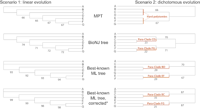
As stated above, the data properties for both scenarios are different. The matrices have a different number of parsimony-informative characters (4 for linear, 2 for dichotomous). Accordingly, the reconstructed optimal trees (here using the maximum parsimony, least-squares, and maximum likelihood criteria), are better resolved / more correct for the linear than for the dichotomous evolution.

MPT = most-parsimonious tree; ML = maximum likelihood. *Corrected for ascertainment bias.

Using all of the variable characters, NJ and ML are generally more decisive and produce higher support for the right branches. But for the dichotomous evolution scenario, they also show ghost-clades ("para-clades" as they include close relatives sharing a recent common origin, but do not represent monophyletic groups sensu Hennig) with low support. The corresponding MPT has no ghost-clades, but it also provides no clues to how B,C,D and E,F,G are related to each other.

Beyond this, and as can be seen in many real-world examples, there is no fundamental difference between character-based inferences such as maximum parsimony (MP) or maximum likelihood (ML) and distance-based inferences (NJ) fulfilling (here) the least-squares criterion (sometimes still called "phenetic" inferences in contrast to the "phylogenetic" parsimony, Bayesian inference and maximum likelihood).

The differences diminish further when we look at the phylograms instead of the cladograms, as shown next.

Another observation we can make is that for the linear-evolution scenario (four synapormophies), the ascertainment bias correction under ML has little effect, but it is crucial for the dichotomous evolution (two synapomorphies) to get sensible branch lengths.

Parsimony provides the most conservative (and least decisive) results for the dichotomous-evolution scenario, also because of the way I applied it: PAUP* allows optimizing trees with hard polytomies when using the default branch-and-bound search (for tree inference as well as bootstrapping), whereas the NJ / BioNJ algorithm and the ML implementation in RAxML will always produce fully dichotomized trees, including zero-length or near-zero-length branches. This explains the difference in the support values of preferred and alternative splits.

(Non-filtered) Bootstrap support consensus networks for the linear evolution scenario. Same scale for all graphs, trivial splits (dashed lines) collapsed.

(Non-filtered) Bootstrap support consensus networks for the dichotomous evolution scenario.

Trees are not wrong, but they miss the point

None of the graphs above show anything strongly erroneous, but they also don't fully capture the evolutionary pathways — that is, the actual ancestor-descendant relationships. This is because our taxon set includes ancestral forms, which, in traditional trees, have to be placed as sisters to part or all of their descendants. Networks provide a quick solution to this limitation.

Median-joining networks inferred with NETWORK 5.0.0.3 for both scenarios, with the inferred (and real) character changes annotated along edges.

Neighbour-nets inferred with SplitsTree 4.13.1 for both scenarios, based on the mean (Hamming) pairwise distances.

The two (perfectly tree-like) graphs, one parsimony-based, the other distance-based, look identical, and place all of the taxa exactly where they should be: the ancestors on the nodes ("medians"), and their (latest) descendants at the tips. But note that in the case of the Neighbour-net this is a visual illusion / approximation: in fact, the ancestors are actually connected by zero-length edges to the node they appear to be sitting on.

Given that both scenarios used here produce trivial, straightforward to interpret, data patterns (see the first figures), the failure of the traditional tree inferences to get it completely right can be a bit unsettling. Trees including primitive-old and derived-new forms are common in the (palaeontological) literature, and typically show many branches lacking high support (note that only ML produced a bootstrap support >90 for a true-tree branch, and only for the linear evolution scenario). To address evolution over time, networks should hence be standard applications, rather than the exception. Cladograms should be long gone, as they show very little beyond the most trivial.

If we want trees (and many of us want trees!), we need tree inferences that can optimize an older taxon on an internal branch or node, to accommodate potentially ancestral forms.

Related blog posts

In Clades, cladograms, cladistics, and why networks are inevitable, I argue that we cannot get around networks when we aim to study taxa from different time scales using their morphologies.

Digging deeper: Population dynamics and individual-based fossil phylogenies raises the question of what we deal with when we use individual fossils (i.e. long-dead individuals) as OTUs in our phylogenetic inferences.
 
Monophyletic groups in networks by David gives an introduction into (fringe) terminology. What to do when dealing with more than a single most-recent common ancestor and past reticulation?

Networks and most recent common ancestors by David discusses the concepts of conservative MRCAs (most recent common ancestors), fuzzy MRCAs and (alternative) LCA — lowest (last) common ancestors in the face of reticulation.

In Stacking neighbour-nets: ancestors and descendants, I outline how one may (and why one should) stack Neighbour-nets to analyse the evolutionary history of a group including (mostly) fossil representatives.

The first Darwinian evolutionary tree[s] show features one rarely finds in a modern-day phylogenetic tree: ancestral and descendant forms, ancestral taxa addressed as species and not higher taxa, and gradual transition between forms (post by David).

Tree metaphors and mathematical trees by David, which introduces János Podani's concept about "branching silhouettes" and how to depict an actual evolutionary tree.

Where have all the ancestors gone? discusses the common notion that we don't have to deal with ancestor-descendant problems in phylogenetics at all, because the scarcity of the (terrestrial) fossil records ensures to only find extinct side (sister) lineages.