Next Generation Sequencing and phylogenetic networks

I have recently been doing a course (along with a bunch of postgraduate students) on Massively Parallel Sequencing, also known as Next Generation Sequencing (NGS). This was a partially successful attempt to teach an old dog some new tricks. More to the point, it has prompted me to think about NGS in relation to phylogenetic networks. Most of the published discussions have focussed on trees, rather than networks.

NGS can potentially provide a fast and cost-effective means of generating multilocus sequence data for phylogenetics (Rannala & Yang 2008; McCormack et al. 2013; Moriarty Lemmon & Lemmon 2013). Unfortunately, the cost for the number of samples typically employed in phylogenetics is currently still beyond the reach of most researchers.

NGS and phylogenetics

Nevertheless, we are sometimes told things like: "The fields of phylogenetics and phylogeography are on the cusp of a revolution, enabled by the rapid expansion of genomic resources and explosion of new genome sequencing technologies." This is probably over-stating the case, as noted by McCormack et al. (2013):

Despite this obvious potential, NGS has been slow to take root in phylogeography and phylogenetics compared to other fields like metagenomics and disease genetics. We suggest that this lag has been caused by four specific aspects of phylogeographic and phylogenetic research: the predominant focus on non-model organisms, the need for sequencing large numbers of samples per species, the lack of consensus regarding library preparation protocols for particular research questions, and the transitional state of the technology (whole-genome data are still neither cost-effective, nor even desirable for phylogeography and phylogenetics, but are paradoxically easier to collect).

Another issue is the historical importance of utilizing gene trees in phylogeography and phylogenetics. Gene trees are most robustly inferred from loci with high information content, for example, a non-recombining locus containing a series of linked SNPs. Individual SNPs, on the other hand, have low information content on a per-locus basis and have been used predominately with classification methods such as Structure and Principal components analysis ... While distance-based genealogies and phylogenies can be built from unlinked SNPs, this ignores models of molecular substitution and probabilistic tree-searching algorithms that have led to more robust phylogenetic inference in the last several decades.

Furthermore, no-one has yet shown that many of the questions currently being asked by phylogeneticists will actually benefit from genomic data. We may well be able to answer some new questions, but that is quite a different thing from a revolution. The essence here is that in science the questions must come first. Collecting data for the sake of it is usually unproductive. So, we need a clear demonstration that genomics is actually needed in phylogenetics (as opposed to other disciplines, where it may indeed be very useful). If increased volume of data will solve a phylogenetic problem then that is good, but there is no necessary reason to expect that it will happen. Statistically, the extra data can lead to improved precision but not necessarily improved accuracy. In science, targeted data collection has always been the most productive approach to any clearly stated experimental question.

For example, the estimated relationships among humans, chimpanzees, and gorillas did not change as a result of genome sampling (Galtier and Daubin 2008), nor did those of malaria species (Kuo et al. 2008), nor those of mammal superorders (Hallström and Janke 2010). (I have discussed the mammal example in a previous blog post: Why are there conflicting placental roots?). In all three cases, the relationships were just as complex after the genome sequencing as before — the resolution of controversial branches in our trees did not occur as a result of increased access to character data.

In this sense, a small sample of representative gene sequences should reveal just as much of the genealogical truth as will a genome-wide sample. A more recent empirical example is presented by O'Neill et al. (2013), who found that including less informative loci added so much noise to the phylogenetic signal that the analysis eventually broke down. The issue here is that as data volume increases so does the potential occurrence of systematic bias due to model mis-specification.

This sort of problem can easily be visualized using phylogenetic networks, in which genome-scale data frequently produce unresolved bushes rather than tree-like phylogenies. I have provided a couple of examples in a previous post (When is there support for a large phylogeny?). Another example is provided by Beiko (2011), which I have reproduced below.

This all suggests that we will need to think carefully about how to apply phylogenetic networks to genome-scale data. Much of the lack of resolution may very well come from the nature of NGS, rather than from the actual evolutionary history.

NGS and networks

There are a number of potential problems with NGS. These may not matter so much for tree-building algorithms, but it is a different matter for networks.

[1]  Increased homoplasy due to sequencing errors
An error rate of even 0.01% is considered good in NGS (eg. Roche 454: 1%; Illumina HiSeq: 0.1%; Life SOLiD: 0.01%), but when this is extrapolated to the genome scale it results in thousands of errors. Networks are sensitive to this magnitude of stochastic error. Indeed, I have already written about the use of phylogenetic networks specifically to identify data errors (Checking data errors with phylogenetic networks).

[2]  Increased homoplasy due to intra-gene processes
These include substitutions, deletions, duplications (especially tandem repeats), inversions, and translocations. These processes can potentially reveal evolutionary history, but we have little idea about how best to process the data in a way that will reveal that history. Currently, we deal with this by lumping most of the processes together as "indels".

[3]  Increased homoplasy due to inter-gene processes
The most common processes known to confound attempts to identify reticulate evolution are incomplete lineage sorting and gene duplication–loss. There are several methods available for addressing these issues in the context of estimating phylogenetic trees, but their applicability to networks is still being assessed.

[4]  Increased homoplasy in non-coding regions
Sanger-style sequencing is usually targeted towards gene-coding regions or their introns, but genome-scale data can include what is currently called "junk DNA". The evolutionary processes in these regions are unknown, as is their applicability to phylogenetic analysis.

[5]  Inadequacies due to data-processing methods
The analysis of NGS data is often a black art — each paper seems to provide its own way of processing the data. This has been a cause of concern expressed in the literature (e.g. Check Hayden 2012; Editorial 2012a, 2012b; MacArthur 2012), especially in the light of the poor documentation and archiving of bioinformatics programs. I have discussed this issue in some previous posts (Poor bioinformatics?; Archiving of bioinformatics software). Perhaps the most talked-about problem is ascertainment bias — there is a brief discussion of this at the end of this post.

Network analysis of NGS data

All of this might make the application of networks to phylogenomics problematic in many cases, because we already have enough challenges dealing with the data from Sanger-style sequencing, without having them be orders of magnitude worse. It will therefore be very interesting to see what emerges from the current attempts to apply phylogenetic networks to NGS data.

There have been a few applications of EDA (exploratory data analysis) programs such as SplitsTree, mostly involving bacteria and viruses, and often in the context of detecting recombination. Not all of these studies have produced networks that look bushy, as shown by the example below (from Söderlund et al. 2013). SplitsTree is mostly limited by the number of samples not by the number of characters, so that genomic data are not a particular analysis issue for algorithms such as neighbor-net. However, you might like to calculate your inter-sample distances outside the program, unless you want the simple p-distance. (Popular genome-scale alternatives include F_st.)

There have also been programs developed for the study of admixture (a.k.a. introgression) in human genomes, such as TreeMix, AdmixTools, and MixMapper, and these might repay wider exploration. I have discussed some of these programs in a previous post (Admixture graphs – evolutionary networks for population biology). Essentially, they first construct a tree and then add reticulations based on various criteria. As is usual with this approach, there is the problem of constructing the initial tree in the presence of reticulation processes, and there seems to be no clear criterion about when to stop adding reticulations — optimization criteria always increase as reticulations are added, so that increasingly complex networks will always be preferred mathematically.

Note — a common data-processing problem

The following explanation of one type of ascertainment bias is adapted from the Fluxus Engineering web site:

For each DNA sample, a large number of short sequences are generated by the NGS sampling. Genomic variants are estimated from the consensus of these NGS sequences, after filtering the sequences for artifacts. Variant lists are never complete — the greater the sequence length, the greater the fraction of the genome that can be sequenced, but there are always uncharted regions which vary from sample to sample. The sampled genome sequences are then compared to a reference genome. NGS software usually reports SNP variants only if they do not match the reference genotype, and if there is sufficient evidence that they are non-reference. Non-reported variants do not necessarily match the reference genotype — they can just as well be sequencing failures, or coverage gaps, or insufficient evidence for a non-reference variant. Networks generated from such data are likely to consist largely of artifacts.

References

Beiko RG (2011) Telling the whole story in a 10,000-genome world. Biology Direct 6: 34.

Check Hayden E (2012) RNA studies under fire. Nature 484: 428.

Editorial (2012a) Must try harder. Nature 483: 509.

Editorial (2012b) Error prone. Nature 487: 406.

Galtier N, Daubin V (2008) Dealing with incongruence in phylogenomic analyses. Philosophical Transactions of the Royal Society of London, Series B: Biological Sciences 363: 4023-4029.

Hallström BM, Janke A (2010) Mammalian evolution may not be strictly bifurcating. Molecular Biology & Evolution 27: 2804-2816.

Kuo C-H, Wares JP, Kissinger JC (2008) The Apicomplexan whole-genome phylogeny: an analysis of incongruence among gene trees. Molecular Biology & Evolution 25: 2689-2698.

Moriarty Lemmon E, Lemmon AR (2013) High-throughput genomic data in systematics and phylogenetics. Annual Review of Ecology, Evolution & Systematics 2013. 44: 19.1–19.23.

MacArthur D (2012) Face up to false positives. Nature 487: 427-428.

McCormack JE, Hird SM, Zellmer AJ, Carstens BC, Brumfield RT (2013) Applications of next-generation sequencing to phylogeography and phylogenetics. Molecular Phylogenetics and Evolution 66: 526-538.

O'Neill EM, Schwartz R, Bullock CT, Williams JS, Shaffer HB, Aguilar-Miguel X, Parra-Olea G, Weisrock DW (2013) Parallel tagged amplicon sequencing reveals major lineages and phylogenetic structure in the North American tiger salamander (Ambystoma tigrinum) species complex. Molecular Ecology 22: 111-129.

Rannala B, Yang Z (2008) Phylogenetic inference using whole genomes. Annual Review of Genomics and Human Genetics 9: 217-231.

Söderlund R, Jernberg C, Källman C, Hedenström I, Eriksson E, Bongcam-Rudloff E, Aspán A (2013) Rapid whole genome sequencing investigation of a familial outbreak of E. coli O121:H19 with a sheep farm as the suspected source. EMBnet Journal 19 suppl.A: 89-90.

World ice hockey champions — a network

The more sports-minded of you will know that Canada and Russia have at least one thing in common — ice hockey. Indeed, Canada dominated the sport at the international level from 1930–1953, and the Soviet Union from 1963–1976, with these two teams being equal rivals during the intervening decade.

The McGill University ice-hockey team in 1881
at the Crystal Palace Rink in Montreal.

Ice hockey is considered to have originated in the eastern parts of Canada, with the first informal rules appearing in 1873. The first organized game of hockey was apparently played on March 3 1875, at the Victoria Skating Rink in Montreal. The first Stanley Cup games were played in 1893; and the National Hockey League (NHL) was formed in 1917.

The first ice hockey games in Europe were played in 1902 at the Prince's Skating Club in Knightsbridge, London. On March 4 1905, Belgium and France played two international games in Brussels. Three years later, the Ligue International de Hockey sur Glace (LIHG) was founded in Paris, with representatives from Belgium, France, Great Britain and Switzerland, and later the same year also from Bohemia (now the Czech Republic). The first LIHG-organized games were played in Berlin, on November 3-5 1908, at which stage Germany also joined.

The 1920 Olympic Summer Games in Antwerp, Belgium, hosted the first international ice hockey tournament with North American participation, and it is from this date that World Championship ice hockey is considered to originate. The first World Championship outside the Olympics took place in 1930, although the Winter Olympics continued to host the Championships until 1972.

The LIHG became the International Ice Hockey Federation (IIHF) in 1954; and it currently has 52 full members, 18 associate members and 2 affiliate members. Only 48 of these members currently compete in the World Championships. It seems worthwhile to explore some of the Championship data, to look at the relative success of the different teams.

World Championships

There have been 77 World Championships between 1930 and 2013, inclusive. The number of teams participating has varied dramatically, with as few as four, due to financial crises, political boycotts, and disputes over professional versus amateur status of the players. For this reason, I have restricted myself solely to the data concerning medal winners (ie. the top three teams).

The data are from Wikipedia. I scored Gold, Silver and Bronze medals as 3, 2 and 1 points, respectively, with 0 points for all other participants. So, the network applies only to those 14 teams that have won at least one medal over the years. I have kept the various teams separate, which means that Czechoslovakia appears along with both Slovakia and the Czech Republic, the Soviet Union appears along with Russia, and both Germany and West Germany are listed.

The network analysis method follows what I have previously used for the FIFA World Cup (soccer). The similarity among the 77 scores for each pair of teams was calculated using the Manhattan distance. A Neighbor-net analysis was then used to display the between-team similarities as a phylogenetic network. Thus, teams that are closely connected in the network are similar to each other based on their overall World Championship results, and those that are further apart are progressively more different from each other.

The network shows the four most successful teams on the left and the less successful teams on the right.

Canada have won 46 medals over the 77 Championships, the Czech Republic (plus Czechoslovakia) has been involved in 12+34=46 medals, Sweden has won 44 medals, and Russia (plus the Soviet Union) has been involved in 8+34=42 medals. So, these four teams have won 178 of the 231 medals (77%). The next best teams are the United States (17 medals), Finland (11) and Switzerland (10). (Note: Slovakia technically has 4+34=38 medals, but the IIHF officially attributes all Czechoslovakian medals to the Czech Republic alone.)

Great Britain won 5 medals in the first 12 Championships, but has won nothing since 1938. The remaining foundation members, Belgium and France, have never won a medal. However, France is still ranked among the 16 teams in the Championship Division, although Great Britain is currently (2013) among the 12 teams in Division I (it was relegated in 1995), and Belgium is among the 12 teams in Division II (relegated in 2005). The other teams currently in the Championship Division that have never won medals are: Denmark, Italy and Norway, plus Belarus, Kazakhstan and Latvia from the former Soviet Union. Austria is the only other medal-winning team not currently in the Championship Division (it was relegated to Division I earlier this year).

World Rankings

The IIHF has provided a World Ranking for 50 of the teams every year since 2003. This provides a more detailed look at the recent history of the various teams (ie. over the past 11 years). The annual ranking is based on the success of the teams in the previous three World Championships plus the most recent Winter Olympics, with each competition being assigned a set number of points and the teams sharing these points based on their finishing position.

I have analyzed these data in the same way as above, except that the data are the actual ranking points awarded to each team each year. I excluded Armenia, Bosnia & Herzegovina, Georgia, Greece, Mongolia and the United Arab Emirates because they were not ranked in all 11 of the years.

The network shows a simple gradient from the most successful teams at the top-left to the least successful teams at the bottom-right. This network arrangement implies that the relative rankings of the teams are very consistent from year to year.

As before, the same four teams have dominated across the past 11 years as they did for all 77 of the Championships (Canada, Sweden, Russia and the Czech Republic) but now also including Finland. These teams are followed by Slovakia, the United States and Switzerland. Only three of these teams have been raked first: Canada and Russia in four years each, and Sweden for three years. However, Sweden is the only team to have been ranked in the top four every year. These same eight teams dominate the current IIHF rankings (2013), with a clear points gap between the eighth and ninth ranked teams.

Note that Switzerland should currently be included in the upper echelon, even though the other teams have been referred to as the "Big Seven". Sadly, in the 2013 World Championships Switzerland won every one of their games except the final, even beating the host nation (Sweden) in their first game; but it is a bit hard to beat the Swedes on their home ice twice in one tournament.

Barcodes, metaphors, and phylogenetic networks

The term "DNA barcoding" is a metaphor, and like all metaphors it is helpful only to the extent that it provides insight into the topic at hand. The metaphor concerns commercial barcodes, which were developed to provide a means of storing and retrieving information about manufactured products. Once a product exists we can create a barcode that uniquely identifies that product. At any future time we can invert this chain of logic, by reading the barcode and thus retrieving information about the product.

Metaphor

Does this metaphor apply in the biological world? Well, partly. Whenever biological variation is discontinuous then we could treat the delimited entities as analogous to products, and some part of the DNA must be unique and could be used as a unique identifier. However, much biological variation is more or less continuous, and at best delimits fuzzy (ie. overlapping) clusters rather than discrete entities; so even the theoretical idea that we could know about biodiversity by reading barcodes is not a forgone conclusion.

Just as importantly, however, barcodes apply to one part of the genome, while biodiversity is about whole organisms and their relationships. Barcodes do not apply to either genomes or organisms, they apply to genes. How many barcodes does a genome need before it is uniquely characterized? A product needs only one, but that is because we defined the product first and then applied the barcode to it. But in biology we read the barcode first and then try to work out what it might apply to.

Furthermore, does barcoding a genome also barcode the organisms? Not that we know of. Each organism is a phenotype, which is a genotype interacting with its environment (in the broadest sense). There is much more to biodiversity then merely a collection of genomes. So, even if we do have a DNA barcode, we don't really know what this tells us about biodiversity.

So, a DNA barcode provides information but not necessarily knowledge, whereas a product barcode provides both. Therein lies the major weakness of the metaphor.

DNA barcoding seems to have started as a means of identifying DNA in foodstuffs, and in this application the metaphor seems to have some use, because the weakness does not have much affect. After all, we are mainly trying to identify DNA that is foreign to the alleged ingredients, which merely asks the question: Is there more to this food item than meets the eye? Since the ingredients are all distinct entities, and we know about them beforehand, all we are doing is identifying the entities by examining their barcodes.

However, DNA barcoding is now being used to help create a catalogue of life, which is a completely different thing. In this application, we are trying to delimit entities based on their alleged barcodes — if they have different barcodes then they thus must be different entities. We are counting barcodes but we are not necessarily counting meaningful biological entities. Here, the metaphorical weakness seems like a major handicap, potentially leading to mis-interpretation of what DNA barcoding can and cannot achieve.

DNA barcoding is a viable technology for helping to quantify DNA diversity, which is what it is used for when examining foodstuffs. But the metaphor should not lead us to the conclusion that information about DNA diversity automatically provides much knowledge about biodiversity as a whole. We would end up with a catalogue, but we would not necessarily know what it refers to. This would be a data-base but it would not be a knowledge-base.

Networks

What does this have to do with phylogenetic networks? Well, the criteria for defining entities and identifying them based on DNA barcodes is usually a phylogenetic tree. We create a phylogenetic tree of the known barcodes, and the closest barcode in the tree is then used as the best "identification" of any newly discovered barcode. Remember, product barcodes are unique by definition, and we know what they refer to. But DNA barcodes are not unique unless we decide that they are; and we have no prior idea what they refer to. We make both decisions with reference to clades on a phylogenetic tree.

But a phylogenetic tree imposes a hierarchical structure on the data, irrespective of whether there actually is such a structure underlying the data. A phylogenetic network might reveal a very different pattern. In particular, when the data are forced into a tree then many of the shared characters become parallelisms and reversals, whereas the network can actually display them as shared characters.

To illustrate this, we can look at some of the data from the first published paper about DNA barcodes:

Hebert PD, Cywinska A, Ball SL, deWaard JR (2003) Biological identifications through DNA barcodes. Proceedings of the Royal Society of London B: Biological Sciences 270: 313-321.

The authors evaluated the usefulness of cytochrome c oxidase I (COI or Cox1) sequences as a barcode. They analyzed sequences 223 amino-acids long from 100 members of the Bilateria. The original analysis was based on Poisson-corrected p-distances and the Neighbour-joining algorithm — chosen because of "its strong track record in the analysis of large species assemblages [and] the additional advantage of generating results much more quickly than alternatives." The tree was shown as rooted on the Platyhelminthes but without explanation (the other two analyses in the same paper had clearly specified outgroups). The tree itself looks like it might have a mid-point root.

No measure of branch support was provided, but the authors concluded that their analysis:

showed good resolution of the major taxonomic groups. Monophyletic assemblages were recovered for three phyla (Annelida, Echinodermata, Platyhelminthes) and the chordate lineages formed a cohesive group. Members of the Nematoda were separated into three groups, but each corresponded to one of the three subclasses that comprise this phylum. Twenty-three out of the 25 arthropods formed a monophyletic group, but the sole representatives of two crustacean classes (Cephalocarida, Maxillopoda) fell outside this group. Twelve out of the 25 molluscan lineages formed a monophyletic assemblage allied to the annelids, but the others were separated into groups that showed marked genetic divergence. One group consisted solely of cephalopods, a second was largely pulmonates and the rest were bivalves.

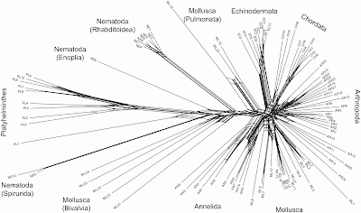
I have tried to reconstruct the data (it is not available online), and re-analyzed it using Neighbor-Net (the closest network equivalent of Neighbour-joining) and uncorrected p-distances.

Some of the recognized taxonomic groups are, indeed, characterized by splits in the network, notably the Echinodermata, the Annelida, the Pulmonata (Mollusca), and the various parts of the Nematoda. However, the other groups are ambiguously defined. In particular, the Chordata, Arthropoda and most of the Mollusca are indistinct based on the gene sequence being analyzed, and there is no split supporting the Bivalvia (Mollusca). There is a split supporting the Platyhelminthes, but it has strong reticulate relationships with parts of the Nematoda — this is unfortunate since this is allegedly the root. Removing sample PL1 from the analysis makes the root a bit less ambiguous, and the network then unites most of the Nematoda as a single group.

This network does not really support the methodology used by the original authors. The authors tested the viability of DNA barcoding by adding a series of "test" sequences, one at a time, to the tree-based analysis, to see whether these sequences clustered with the "correct" group in the tree. However, most of the sequences don't form clear groups in the network, so it is not obvious how one would unambiguously decide which alleged group each test sequence clusters with.

The barcode metaphor looks very poor in this network. I wonder whether DNA barcoding would have taken off if the authors had presented this network rather than their original tree?

Phylogenetics with SpongeBob

Some time ago I published a blog post on Faux phylogenies in which I included a phylogeny of cartoon animals by Mike Keesey. In this phylogeny, SpongeBob SquarePants was the outgroup. However, SpongeBob goes much further than this.

Importantly, the main characters in the cartoon have representative members of several phyla (notably, except the Cnidaria). Indeed, the List of SpongeBob SquarePants characters at Wikipedia makes this very clear. This opens up the possibility that they could be a means of using modern culture to introduce phylogenetics. This idea has been independently discovered at least twice.

Perhaps the best known usage is by Paul Arriola, produced for his freshman biology students, as shown in the first figure.

This has been reproduced in several places on the web, including Pinterest (e.g. here and here), Facebook (e.g. here and here), and academia (here).

Another, apparently independent, usage is by Rita Chen of the sister artists known as The Hurricanes.

Note that a few "extra" characters have been added (the planarian, ragworm and roundworm), and that the names are not all quite correct.

By the way, did you know that there is a species of sponge-like fungus (in the Boletaceae) called Spongiforma squarepantsii, and named after the character? If not, then see Wikipedia.

What are evolutionary networks currently used for?

These days, there are many unrooted affinity-type networks used to display conflicting phylogenetic signals. There are many different methods available, although the various forms of splits graphs seem to dominate, especially NeighborNet and Consensus Networks (for species-level data), and Reduced Median Networks and Median Joining Networks (for population-level data). However, phylogeneticists are interested in genealogies, not just data displays.

Unfortunately, rooted evolutionary networks are not so well off. There is a great need for such networks in phylogenetics, but there are very few automated methods available for constructing them. These networks are needed whenever a genealogy involves reticulation processes rather than solely divergence. The latter produces a tree-like evolutionary history but the former do not, and these thus require network methods.

Due to the lack of obvious methods, most current research papers still do not illustrate reticulate evolution with a genealogy. A collection of ad hoc methods is usually applied to the data, and the evolutionary processes are then inferred from this. However, the use of a network to illustrate the inferred genealogy is rather rare.

Indeed, for species-level studies most papers simply present a set of incongruent gene trees, although some of them also illustrate either (i) the tree derived from the combined data, or (ii) a consensus tree with or without the conflicting relationships, or (iii) a pair of cophylogeny trees. Occasionally, the hybrid origin of some of the species, for example, is illustrated, but the putative parents are not connected in a phylogeny.

Population-level studies often present unrooted haplotype networks, illustrating processes such as hybridization and introgression between closely related species, or the evolution of domesticated species.

However, these ad hoc methods do not mean that evolutionary networks do not appear in the literature. In this blog post I include a representative sample of rooted networks that are intended to illustrate inferred genealogies. They are grouped according to the evolutionary processes being studied (see Reticulation patterns and processes in phylogenetic networks). I have also briefly indicated how the networks were constructed.

Homoploid Hybridization

Hybridization is commonly studied in the literature, and phylogenetic networks appear not infrequently. This first example was constructed by the unreleased program HyperPars.

Dickerman AW (1998) Generalizing phylogenetic parsimony from the tree to the forest. Systematic Biology 47: 414-426.

This next example was constructed by program SplitsTree. Note that the root of the network is not clearly indicated.

Pirie MD, Humphreys AM, Barker NP, Linder HP (2009) Reticulation, data combination, and inferring evolutionary history: an example from Danthonioideae (Poaceae). Systematic Biology 58: 612-628.

This example was constructed manually from a set of gene trees. Note that it is drawn in a rather unusual style for indicating hybridization.

Sang T, Crawford D, Stuessy T (1997) Chloroplast DNA phylogeny, reticulate evolution, and biogeography of Paeonia (Paeoniaceae). American Journal of Botany 84: 1120-1136.

Polyploid Hybridization

Polyploid hybridization is probably the most likely type of study to have a phylogenetic network. This is at least partly because there is a computer program, Padre, to automate much of the work. This program was used to construct this first network.

Marcussen T, Jakobsen KS, Danihelka J, Ballard HE, Blaxland K, Brysting AK, Oxelman B (2012) Inferring species networks from gene trees in high-polyploid North American and Hawaiian violets (Viola, Violaceae). Systematic Biology 61: 107-126.

This next example was also constructed by program Padre.

Sessa EB, Zimmer EA, Givnish TJ (2012) Unraveling reticulate evolution in North American Dryopteris (Dryopteridaceae). BMC Evolutionary Biology 12: 104.

This example constructed manually from a gene tree.

Marhold K, Lihová J (2006) Polyploidy, hybridization and reticulate evolution: lessons from the Brassicaceae. Plant Systematics and Evolution 259: 143-174.

Introgressive Hybridization

Introgression is a widely studied phenomenon. However, rooted evolutionary networks are rarely presented. This first one was constructed manually from a set of gene trees.

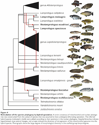
Koblmüller S, Duftner N, Sefc KM, Aibara M, Stipacek M, Blanc M, Egger B, Sturmbauer C (2007) Reticulate phylogeny of gastropod-shell-breeding cichlids from Lake Tanganyika — the result of repeated introgressive hybridization. BMC Evolutionary Biology 7: 7.

The next example was also constructed manually from a set of gene trees.

Morgan DR (2003) nrDNA external transcribed spacer (ETS) sequence data, reticulate evolution, and the systematics of Machaeranthera (Asteraceae). Systematic Botany 28: 179-190.

This example was constructed by program SplitsTree.

Labate JA, Robertson LD (2012) Evidence of cryptic introgression in tomato (Solanum lycopersicum L.) based on wild tomato species alleles. BMC Plant Biology 12: 133.

Horizontal Gene Transfer

HGT is a hot topic these days, both among prokaryotes and among eukaryotes, although most papers do not present a phylogenetic network. The first example was constructed by program Sprit from the species tree and a gene tree.

Walsh AM, Kortschak RD, Gardner MG, Bertozzi T, Adelson DL (2013) Widespread horizontal transfer of retrotransposons. Proceedings of the National Academy of Sciences USA 110: 1012-1016.

This next example was constructed manually from a gene tree.

Delwiche CF, Palmer JD (1996) Rampant horizontal transfer and duplication of rubisco genes in eubacteria and plastids. Molecular Biology and Evolution 13: 873-882.

This example was constructed manually from incongruence among a series of gene trees.

Richards TA, Soanes DM, Foster PG, Leonard G, Thornton CR, Talbot NJ (2009) Phylogenomic analysis demonstrates a pattern of rare and ancient horizontal gene transfer between plants and fungi. The Plant Cell 21: 1897-1911.

Homologous Recombination

Intra-genic recombination is often studied without reference to a network. Nevertheless, several programs exist, and this particular network was constructed by program Kwarg.

Jenkins PA, Song YS, Brem RB (2012) Genealogy-based methods for inference of historical recombination and gene flow and their application in Saccharomyces cerevisiae. PLoS One 7: e46947.

Chromosomal rearrangements are studied rather rarely. This network was constructed manually from a phylogenetic tree. Note that the root of the network is not clearly indicated.

Rumpler Y, Hauwy M, Fausser JL, Roos C, Zaramody A, Andriaholinirina N, Zinner D (2011) Comparing chromosomal and mitochondrial phylogenies of the Indriidae (Primates, Lemuriformes). Chromosome Research 19: 209-224.

Viral Reassortment

Reassortment of segmented viruses produces very complex networks. This one is a partial network, constructed manually from a series of phylogenetic analyses.

Smith GJ, Vijaykrishna D, Bahl J, Lycett SJ, Worobey M, Pybus OG, Ma SK, Cheung CL, Raghwani J, Bhatt S, Peiris JS, Guan Y, Rambaut A (2009) Origins and evolutionary genomics of the 2009 swine-origin H1N1 influenza A epidemic. Nature 459(7250): 1122-1125.

Genome Fusion

This is a difficult topic to study. As is almost always done, this network was constructed manually from a phylogenetic tree.

Thiergart T, Landan G, Schenk M, Dagan T, Martin WF (2012) An evolutionary network of genes present in the eukaryote common ancestor polls genomes on eukaryotic and mitochondrial origin. Genome Biology and Evolution 4: 466-485.

Apomixis

This topic rarely involves networks. This network was constructed manually from the output of program SplitsTree.

Dyer RJ, Savolainen V, Schneider H (2012) Apomixis and reticulate evolution in the Asplenium monanthes fern complex. Annals of Botany 110: 1515-1529.

Removing Convergence

This is an unusual use of a network, but the author notes that "the use of reticulations clarifies the phylogeny by factoring out apparent convergence, even though there is no reason to think that actual hybridization or introgression has occurred." The network was constructed by an unreleased program.

Alroy J (1995) Continuous track analysis: a new phylogenetic and biogeographic method. Systematic Biology 44: 152-178.

Whither phylogenetics?

Some time ago I published a blog post in which I used Google's Ngram Viewer to explore some of the history of phylogenetic nertworks (Ngrams and phylogenetics). Today I use Google Trends to look at the worldwide popularity of some phylogenetic terms in Google's web searches.

The data start in January 2004 and end in September 2013. According to Google, the vertical axis "numbers represent search interest relative to the highest point on the chart. If, at most, 10% of searches for the given region and time frame were for "pizza", then we'd consider this 100."

The first search term is for "Phylogenetics", which shows a depressing trend.

The next term is "Phylogeny", which shows the same trend.

The final term is "Phylogenetic Tree", which looks somewhat better.

Either the people have lost interest in phylogenetics, or they already know about it so they no longer need to do web searches to find out about it.

Mis-interpreting splits graphs

I have written before about the interpretation of splits graphs, and provided a simple worked example (How to interpret splits graphs). However, it seems to be worth re-emphasizing the issue here, as I have recently had a paper drawn to my attention that incorrectly infers "groups" of genes from a series of splits graphs.

The essential point to understand is that splits graphs are separation networks. That is, the edges in the graph represent separation between two clusters of nodes in the network; or, they split the graph in two. Formally, each edge (or set of parallel edges) represents a bipartition (or split) of the taxa/genes based on one or more characteristics.

Therefore, the only groups of nodes that are "supported" by a network are those that are represented by splits in the graph, or by some unique combination of splits.

I will illustrate this using the paper already mentioned:

Marz M, Kirsten T, Stadler PF (2008) Evolution of spliceosomal snRNA genes in metazoan animals. Journal of Molecular Evolution 67: 594-607.

The authors describe their analyses thus:

We use split decomposition and the neighbor net algorithm (as implemented as part of the SplitsTree4 package) to construct phylogenetic networks rather than phylogenetic trees. The advantage of these method is that they are very conservative and that the reconstructed networks provide an easy-to-grasp representation of the considerable noise in the sequence data.

Unfortunately, it is not clear which network algorithm was used for the networks actually presented in the paper. However, this does not affect the interpretation of the graphs (only the number of splits shown).

For Figure 1, the authors claim:

A phylogenetic analysis of the individual snRNA families, nevertheless, does not show widely separated paralogue groups that are stable throughout larger clades. Figure 1, for example, shows that the U5 variants described in Chen et al. (2005) do not form clear paralogue groups beyond the closest relatives of Drosophila melanogaster. On the other hand, there is some evidence for distinguishable paralogues outside the melanogaster subgroup.

This interpretation of Figure 1 seems to be quite reasonable.

However, for Figure 2 they claim:

The situation is much clearer for the drosophilid U4 snRNAs, where three paralogue groups can be distinguished (see Fig. 2). One group is well separated from the other two and internally rather diverse. The other two groups are very clearly distinguishable for the melanogaster and obscura group (see Drosophila 12 Genomes Consortium 2007). For D. virilis, D. mojavensis, D. grimshawi, and D. willistoni we have two nearly identical copies instead of two different groups of genes.

In Figure 2 (which is labelled as a "phylogenetic tree"), only the recognition of "group 1" is very well supported by a split in the network (ie. there is a long set of edges separating the "group 1" genes from the rest of the genes). The distinction between "group 2" and "group 3" does not correspond to any split in the network, although there are a few splits in the network shown that could be used to recognize groups (notably the "wi" genes).

Furthermore, for Figure 3 the authors claim:

In teleost fish, we find clearly recognizable paralogue groups for U2, U4, and U5 snRNAs. Surprisingly, the medaka Oryzias latipes has only a single group of closely related sequences, despite the fact that for U4, the split of the paralogues appear to predate the last common ancestor of zebrafish and fugu (Fig. 3).

However, in Figure 3: the left-hand network shows three lines that allegedly define groups, only two of which are supported by splits; the middle network shows three lines that define groups, only one of which is supported by a split; and the right-hand network shows two lines that define groups, neither of which is supported by a split. Once again, there are splits in these networks that do form groupings. For example, in the third network, one of the largest splits supports a grouping of the "bfl" genes, while the other supports a grouping of "bfl" + "pma".

Thus, it seems that the authors' recognition of various paralogue groups is at not well supported by their network analyses. Nevertheless, there are reasonably well-supported splits in the networks shown, which therefore could be used to recognize groups, if desired.

A network analysis of airplane disasters

I hate heights. This is a well-known syndrome (acrophobia), and so I am not alone. However, it does mean that I dislike being in airplanes, especially small ones. In turn, this means that I am interested in air disasters, because it gives me a very good reason to feel that I should dislike being in planes.

Airplane crashes are publicly documented in a way that car crashes, for example, are not. The latter are all too common, sadly, and so you will not find any lists online detailing them. You will, however, find plenty of information about airplane crashes, including a lot of details that you might be better off not knowing about. I will skip most of these morbid details, since this is a family blog, but in this post I will be looking at some of the actual data.

The only airline never to have been involved in a fatal accident in the jet age.

Airplane incidents

One internet site that you might like to peruse is the Aviation Safety Network. which has a database with details of all known aviation incidents worldwide. From 2 August 1919 to 1 October 2013, there were 16,844 recorded incidents, including 13,785 accidents, 1,045 hijackings, and 708 other criminal occurrences.

The information is mostly taken from the reports that arise from the official investigations (if there was one). If you read some of the descriptions, not only will you never fly again, you will never even set foot in another airborne conveyance, even while it is still on the ground. What this database does is itemize every single thing that could possibly go wrong with a plane, and what effect this has on the people in it.

There is a long-standing rumour that the most dangerous parts of a flight are take off and landing. However, the data make it clear that this is complete nonsense. Consider, for example, the circumstances of the 40 worst accidents in terms of number of fatalities per plane (excluding ground fatalities):

Taxi phase Take off phase Initial climb phase En route phase Approach phase Landing phase

1 2 1  24 9 3

If all planes ever did was take off and then immediately land, the passengers and crew would all be much better off.

However, the worst double-accident did occur while one plane was taxiing and another was taking off. Both were Boeing 747s, and their collision killed 335 of the 396 people in the taxiing plane and all 248 people in the plane that was taking off. This was in the Canary Islands in 1977.

The worst accident involving a single plane occurred in Japan in 1985, when 520 of 524 people died. The 747 plane had previously suffered damage, which apparently was not repaired properly, and the plane therefore ruptured in mid-air. [Note: 747s on domestic routes in Japan are configured to carry close to the maximum number of passengers.] The next worst accident (all 346 people died) occurred when the luggage compartment of a DC-10 opened shortly after taking off in France in 1974.

And so the list goes on, usually involving the failure of some part of the aircraft systems. However, an all too common cause of fatal airplane accidents is what is euphemistically called Controlled Flight Into Terrain (CFIT), which means that the pilot was in control of an undamaged plane at the time of the crash. This problem has been partly addressed by the introduction of Traffic Collision Avoidance Systems (TCAS) and Minimum Safe Altitude Warning (MSAW) devices.

Actually, when you look at it, 35 of the top 40 accidents occurred from 1972 to 1999, inclusive. Only 5 of them occurred after that, and none of them after June 2009. So, air safety is officially considered to be improving continuously through time. Prior to 1970, when the Boeing 747 was introduced, accidents involved fewer people because there were far fewer passengers per plane. [The original 747 had 2.5 times the capacity of the previous Boeing 707.] So, only two accidents from the 1960s make it even into the top 100 list, and none of them were prior to 1962.

A network

The Aviation Safety Network site also provides summary lists concerning some of the accident situations, and it is this summary information that we are considering here. In particular, we are interested in the information regarding the nature of the flights. The data are the number of fatal hull-loss accidents (fuselage written off, damaged beyond repair) per year and the number of associated fatalities. The data cover the years 1942 to 2012, inclusive (71 years).

The flight categories include: Training flight (total of 136 accidents and 553 casualties over the 71 years), Ferry / positioning activity (137 accidents, 523 casualties), Cargo flight (712; 2,986), International scheduled passenger flight (367; 17,597), and Domestic scheduled passenger flight (1,299; 39,403). For the Training flights, Ferrying, and Cargo flights, this is an average of ~4 casualties per accident; for the Domestic passenger flights it is ~30 casualties per accident; and for the International passenger flights it is ~48 casualties per accident. [The summary data for both the International and Domestic Non-Scheduled Passenger flights are missing from the web site.]

I have analyzed the annual accident data using a phylogenetic network as a tool for exploratory data analysis. To create the network, I first calculated the similarity of the years using the Manhattan distance, and a Neighbor-net analysis was then used to display the between-year similarities as a phylogenetic network. So, years that are closely connected in the network are similar to each other based on the number and severity of the aircraft accidents, and those that are further apart are progressively more different from each other.

Basically, the accidents increase in number and severity from top to bottom in the network, with 1985 (see above) and 1972 being the worst years. The worst period was 1969-1980 (shown in purple), with one exception (1975). Note that 1977 was overall not a particularly bad year, in spite of the Canary Islands incident (see above).

Perhaps the most important message in the network is that the years 2000-2012 (in red) are generally clustered with the 1940s (green) and 1950s (blue). So, in spite of the massively greater volume of air traffic in this century, the number of fatal accidents is currently not much greater than it was before the advent of the jet age.

The years 2000, 2001 and 2009 are clustered away from the others (at the top left) because there were still a few bad accidents involving International flights even though the number of accidents involving Domestic flights was low. Indeed, 2000-2001 were the first years to return to the Domestic accident levels of 1942-1945 (which are clustered at the top right).

I presume that I should take great comfort from this overall trend. The reason for it is not hard to fathom, and indeed it is the purpose of the Aviation Safety Network. Every time there is a reported aviation incident it is investigated, and any lessons learned are disseminated. So, if the circumstances leading to an incident are avoidable, either by improving the technology or by changing the human operating procedures, then efforts are made by the authorities to implement those changes, so that the incidents will not be repeated. Safety must therefore increase, at least until radically different modes of transport are introduced. This is why the 1970s were so dangerous — the aviation authorities were suddenly confronted with the consequences of having jumbo jets in the skies.

This is the fundamental difference from car accidents, of course. On the ground, we insist on repeating the same types of incidents over and over again, with only improvements in technology to help us. The human operating procedures remain essentially the same, and fallable. I guess that is why car manufacturers have been developing Advanced Driver Assistance Systems (ADAS), as a step towards semi- or fully autonomous vehicles.

Reticulation patterns and processes in phylogenetic networks

When it comes to phylogenetic networks, there is often misunderstanding between biological and computational scientists, because the former tend to focus on the biological processes underlying the network whereas the latter focus on the patterns needing to be analyzed to produce the networks.

Here, I try to provide a summary of the different processes and patterns involved in reticulation, so that both "sides" get an overview, and hopefully can communicate more easily. I am principally discussing the development of networks that display evolutionary history.

In phylogenetics, historical processes create contemporary patterns, and we then try to detect those patterns, and assess them in order to determine what process created each pattern. Computationally, algorithms will detect certain data patterns and display them in a directed acyclic graph, which is then interpreted biologically. What needs to happen is for us to identify the possible patterns created by the different processes, so that algorithms can be developed that will detect them. It is doubtful that an algorithm will be able to identify all individual processes — it will be up to biologists to work out what process created each pattern detected.

In what follows, there are major simplifications from both the biological and computational points of view, so please be aware of that. In particular, note that I have not discussed either deep coalescence or gene duplication-loss which, if present, will confound the detection of reticulation patterns.

Hybridization (hybrid speciation)

This is the formation of a new species via sexual reproduction. There are two basic forms that are of interest:
Homoploid Hybridization, in which one copy of the genome is inherited from each parent species (eg. diploid parents create a diploid hybrid);
Polyploid Hybridization, in which multiple copies of the genome are inherited from each parent species (eg. diploid parents create a polyploid hybrid).

Polyploid hybridization is usually assessed by sequencing each copy of the genome in the hybrid species, and treating each copy as a terminal in the data analysis, This produces a multi-labelled genome tree, which is then turned into a single-labelled species network.

At the species level, homoploid hybridization is usually assessed by sequencing several genes in the hybrid species (often from both the nuclear and non-nuclear genomes) and producing independent gene trees. The species network is created by resolving conflicts among the gene trees. This form of analysis assumes a data pattern that is very similar to that of HGT.

In population studies, homoploid hybridization is usually assessed at the sequence level, using multiple-copy nuclear genes, where hybrids are detected by additive polymorphisms at some alignment positions.

Introgression (introgressive hybridization)

This is the transfer of genetic material from one species to another via sexual reproduction. This happens when hybrid individuals back-cross preferentially to one of the parental species, rather than forming a new hybrid species. It can involve anything from 1-49% of the genome (at 50% it is best called hybridization). The data pattern created is very similar to that of HGT (the transfer of genetic material from one species to another via non-sexual means).

It is usually assessed at the population level, by sequencing one or more genes (often from both the nuclear and non-nuclear genomes) from many individuals, and demonstrating that identical haplotypes (haploid genotypes) occur in what are recognized as separate species. This is done by constructing a haplotype network. Often, individuals are detected where the non-nuclear haplotype differs from the nuclear haplotype (as shown in the figure).

Horizontal Gene Transfer

This is the transfer of genetic material from one species to another via non-sexual means (eg. transformation, transduction, or conjugation). The data pattern created is very similar to that of introgression (the transfer of genetic material from one species to another via sexual reproduction).

It is sometimes assessed by sequencing several genes and producing independent gene trees. The species network is created by resolving conflicts among the gene trees. This form of analysis assumes data that are very similar to those of homoploid hybridization or recombination.

Alternatively, it is often assessed by comparing gene trees to a species tree (either pre-specified, or derived from multi-gene data). The species network is created by resolving conflicts between the gene trees and the species tree.

Homologous Recombination and Viral Reassortment

These involve homologous parts of a genome breaking part and re-arranging themselves, often during sexual reproduction. With cross-over the two genomes exchange material, and with gene conversion one genome acquires material from the other. There are three basic forms that are of interest:
Intra-genic Recombination, in which the break-points occur within a single gene;
Inter-genic Recombination, in which the break-points occur in different genes or non-coding spaces between genes;
Reassortment, in which segmented viruses re-combine their segments to create new strains (similar to gene conversion); this is basically inter-genic recombination without sex.

Intra-genic recombination is usually analyzed at the sequence level, based on ordered data. The gene network is constructed by identifying break-points, and thus the recombined segments. It is also possible for one of the donors of a recombined sequence to be missing from the dataset, in which case the data pattern will be the same as for HGT without the donor sampled.

Inter-genic recombination will produce the same pattern as hybridization, if both break-points are outside the region sequenced. Furthermore, homoploid hybridization can be thought of as recombination of whole chromosomes.

Viral reassortment is usually assessed by comparing strains with each other based on presence-absence of segmental haplotypes (rather similar to haplotyping of sexual organisms). This is a unique form of analysis, and it can produce incredibly complex networks.

Summary

Process Polyploid hybridization (species) Homoploid hybridization (species) Homoploid hybridization (population) Introgression (population) Horizontal gene transfer (species) Intra-genic recombination Inter-genic recombination Reassortment (population)

Evaluation method multi-labelled tree incongruent gene trees sequence additive polymorphisms haplotype network incongruent gene trees incongruent gene/species trees sequence break-points incongruent gene trees haplotype network

It may be impossible ever to reliably distinguish homoploid hybridization, introgression, HGT and inter-genic recombination from each other by pattern analysis alone, at least not without genome-scale data.