Typology of semantic promiscuity (Open problems in computational diversity linguistics 10)

The final problem in my list of ten open problems in computational diversity linguistics touches upon a phenomenon that most linguists, let alone ordinary people, might not have even have heard about. As a result, the phenomenon does not have a real name in linguistics, and this makes it even more difficult to talk about it.

Semantic promiscuity, in brief, refers to the empirical observations that: (1) the words in the lexicon of human languages are often built from already existing words or word parts, and that (2) the words that are frequently "recycled", ie. the words that are promiscuous (similar to the sense of promiscuous domains in biology, see Basu et al. 2008) denote very common concepts.

If this turns out to be true, that the meaning of words decides, at least to some degree, their success in giving rise to new words, then it should be possible to derive a typology of promiscuous concepts, or some kind of cross-linguistic ranking of those concepts that turn out to be the most successful on the long run.

Our problem can (at least for the moment, since we still have problems of completely grasping the phenomenon, as can be seen from the next section) thus be stated as follows:

Assuming a certain pre-selection of concepts that we assume are expressed by as many languages as possible, can we find out which of the concepts in the sample give rise to the largest amount of new words?

I am not completely happy with this problem definition, since a concept does not actually give rise to a new word, but instead a concept is expressed by a word that is then used to form a new word; but I have decided to leave the problem in this form for reasons of simplicity.

Background on semantic promiscuity

The basic idea of semantic promiscuity goes back to my time as a PhD student in Düsseldorf. My supervisor then was Hans Geisler, a Romance linguist, with a special interest in sound change and sensory-motor concepts. Sensory-motor concepts are concepts that are thought to be grounded in sensory-motor processes. In concrete, scholars assume that many abstract concepts expressed by many, if not all, languages of the world originate in concepts that denote concrete bodily experience (Ströbel 2016).

Thus, we can "grasp an idea", we can "face consequences", or we can "hold a thought". In such cases we express something that is abstract in nature, but expressed by means of verbs that are originally concrete in their meaning and relate to our bodily experience ("to grasp", "to face", "to hold").

When I later met Hans Geisler in 2016 in Düsseldorf, he presented me with an article that he had recently submitted for an anthology that appeared two years later (Geisler 2018). This article, titled "Sind unsere Wörter von Sinnen?" (approximate translation of this pun would be: "Are our words out of the sense?"), investigates concepts such as "to stand" and "to fall" and their importance for the lexicon of German language. Geisler claims that it is due to the importance of the sensory-motor concepts of "standing" and "falling" that words built from stehen ("to stand") and fallen ("to fall") are among the most productive (or promiscuous) ones in the German lexicon.

Words built from fallen and stehen in German.

I found (and still find) this idea fascinating, since it may explain (if it turns out to hold true for a larger sample of the world's languages) the structure of a language's lexicon as a consequence of universal experiences shared among all humans.

Geisler did not have a term for the phenomenon at hand. However, I was working at the same time in a lab with biologists (led by Eric Bapteste and Philippe Lopez), who introduced me to the idea of domain promiscuity in biology, during a longer discussion about similar processes between linguistics and biology. In our paper reporting our discussion of these similarities, we proposed that the comparison of word formation processes in linguistics and protein assembly processes in biology could provide fruitful analogies for future investigations (List et al. 2016: 8ff). But we did not (yet) use the term promiscuity in the linguistic domain.

Geisler's idea, that the success of words to be used to form other words in the lexicon of a language may depend on the semantics of the original terms, changed my view on the topic completely, and I began to search for a good term to denote the phenomenon. I did not want to use the term "promiscuity", because of its original meaning.

Linguistics has the term "productive", which is used for particular morphemes that can be easily attached to existing words to form new ones (eg. by turning a verb into a noun, or by turning a noun into an adjective, etc.). However, "productivity" starts from the form and ignores the concepts, while concepts play a crucial role for Geisler's phenomenon.

At some point, I gave up and began to use the term "promiscuity" in lack of a better term, first in a blogpost discussing Geisler's paper (List 2018, available here). Later in 2018, Nathanael E. Schweikhard, a doctoral student in our research group, developed the idea further, using the term semantic promiscuity (Schweikhard 2018, available here), which considers my tenth and last open problem in computational diversity linguistics (at least for 2019).

In the discussions with Schweikhard, which were very fruitful, we also learned that the idea of expansion and attraction of concepts comes close to the idea of semantic promiscuity. This references Blank's (2003) idea that some concepts tend to frequently attract new words to express them (think of concepts underlying taboo, for simplicity), while other concepts tend to give rise to many new words ("head" is a good example, if you think of all the meanings it can have in different concepts),. However, since Blank is interested in the form, while we are interested in the concept, I agree with Schweikhard in sticking with "promiscuity" instead of adopting Blank's term.

Why it is hard to establish a typology of semantic promiscuity

Assuming that certain cross-linguistic tendencies can be found that would confirm the hypothesis of semantic promiscuity, why is it hard to do so? I see three major obstacles here: one related to the data, one related to annotation, and one related to the comparison.

The data problem is a problem of sparseness. For most of the languages for which we have lexical data, the available data are so sparse that we often even have problems to find a list of 200 or more words. I know this well, since we were struggling hard in a phylogenetic study of Sino-Tibetan languages, where we ended up discarding many interesting languages because the sources did not provide enough lexical data to fill in our wordlists (Sagart et al. 2019).

In order to investigate semantic promiscuity, we need substantially more data than we need for phylogenetic studies, since we ultimately want to investigate the structure of word families inside a given language and compare these structures cross-linguistically. It is not clear where to start here, although it is clear that we cannot be exhaustive in linguistics, as biologists can be when sequencing a whole gene or genome. I think that one would need, at least, 1,000 words per language in order to be able to start looking into semantic promiscuity.

The second problem points to the annotation and the analysis that would be needed in order to investigate the phenomenon sufficiently. What Hans Geisler used in his study were larger dictionaries of German that are digitally available and readily annotated. However, for a cross-linguistic study of semantic promiscuity, all of the annotation work of word families would still have to be done from scratch.

Unfortunately, we have also seen that the algorithms for automated morpheme detection that have been proposed today usually fail greatly when it comes to detecting morpheme boundaries. In addition, word families often have a complex structure, and parts of the words shared across other words are not necessarily identical, due to numerous processes involved in word formation. So, a simple algorithm that splits the words into potential morphemes would not be enough. Another algorithm that identifies language-internal cognate morphemes would be needed; and here, again, we are still waiting for convincing approaches to be developed by computational linguists.

The third problem is the comparison itself, reflects the problem of comparing word-family data across different languages. Since every language has its own structure of words and a very individual set of word families, it is not trivial to decide how one should compare annotated word-family data across multiple languages. While one could try to compare words with the same meaning in different languages, it is quite possible that one would miss many potentially interesting patterns, especially since we do not yet know how (and if at all) the idea of promiscuity features across languages.

Traditional approaches

Apart from the work by Geisler (2018), mentioned above, we find some interesting studies on word formation and compounding in which scholars have addressed some similar questions. Thus, Steve Pepper has submitted (as far as I know) his PhD thesis on The Typology and Semantics of Binomial Lexemes (Pepper 2019, draft here), where he looks into the structure of words that are frequently constructed from two nominal parts, such as "windmill", "railway", etc. In her masters thesis titled Body Part Metaphors as a Window to Cognition, Annika Tjuka investigates how terms for objects and landscapes are created with help of terms originally denoting body parts (such as the "foot" of the table, etc., see Tjuka 2019).

Both of these studies touch on the idea of semantic promiscuity, since they try to look at the lexicon from a concept-based perspective, as opposed to a pure form-based one, and they also try to look at patterns that might emerge when looking at more than one language alone. However, given their respective focus (Pepper looking at a specific type of compounds, Tjuka looking at body-part metaphors), they do not address the typology of semantic promiscuity in general, although they provide very interesting evidence showing that lexical semantics plays an important role in word formation.

Computational approaches

The only study that I know of that comes close to studying the idea of semantic promiscuity computationally is by Keller and Schulz (2014). In this study, the authors analyze the distribution of morpheme family sizes in English and German across a time span of 200 years. Using Birth-Death-Innovation Models (explained in more detail in the paper), they try to measure the dynamics underlying the process of word formation. Their general finding (at least for the English and German data analyzed) is that new words tend to be built from those word forms that appear less frequently across other words in a given language. If this holds true, it would mean that speakers tend to avoid words that are already too promiscuous as a basis to coin new words for a given language. What the study definitely shows is that any study of semantic promiscuity has to look at competing explanations.

Initial ideas for improvement

If we accept that the corpus perspective cannot help us to dive deep into the semantics, since semantics cannot be automatically inferred from corpora (at least not yet to a degree that would allow us to compare them afterwards across a sufficient sample of languages), then we need to address the question in smaller steps.

For the time being, the idea that a larger amount of the words in the lexicon of human languages are recycled from words that originally express specific meanings remains a hypothesis (whatever those meanings may be, since the idea of sensory motor concepts is just one suggestion for a potential candidate for a semantic field). There are enough alternative explanations that could drive the formation of new words, be it the frequency of recycled morphemes in a lexicon, as proposed by Keller and Schulz, or other factors that we still not know, or that I do not know, because I have not yet read the relevant literature.

As long as the idea remains a hypothesis, we should first try to find ways to test it. A starting point could consist of the collection of larger wordlists for the languages of the world (eg. more than 300 words per language) which are already morphologically segmented. With such a corpus, one could easily create word families, by checking which morphemes are re-used across words. By comparing the concepts that share a given morpheme, one could try and check to which degree, for example, sensory-motor concepts form clusters with other concepts.

All in all, my idea is far from being concrete; but what seems clear is that we will need to work on larger datasets that offer word lists for a sufficiently large sample of languages in morpheme-segmented form.

Outlook

Whenever I try to think about the problem of semantic promiscuity, asking myself whether it is a real phenomenon or just a myth, and whether a typology in the form of a world-wide ranking is possible after all, I feel that my brain is starting to itch. It feels like there is something that I cannot really grasp (yet, hopefully), and something I haven't really understood.

If the readers of this post feel the same way afterwards, then there are two possibilities as to why you might feel as I do: you could suffer from the same problem that I have whenever I try to get my head around semantics, or you could just have fallen victim of a largely incomprehensible blog post. I hope, of course, that none of you will suffer from anything; and I will be glad for any additional ideas that might help us to understand this matter more properly.

References

Basu, Malay Kumar and Carmel, Liran and Rogozin, Igor B. and Koonin, Eugene V. (2008) Evolution of protein domain promiscuity in eukaryotes. Genome Research 18: 449-461.

Blank, Andreas (1997) Prinzipien des lexikalischen Bedeutungswandels am Beispiel der romanischen Sprachen. Tübingen:Niemeyer.

Geisler, Hans (2018) Sind unsere Wörter von Sinnen? Überlegungen zu den sensomotorischen Grundlagen der Begriffsbildung. In: Kazzazi, Kerstin and Luttermann, Karin and Wahl, Sabine and Fritz, Thomas A. (eds.) Worte über Wörter: Festschrift zu Ehren von Elke Ronneberger-Sibold. Tübingen:Stauffenburg. 131-142.

Keller, Daniela Barbara and Schultz, Jörg (2014) Word formation is aware of morpheme family size. PLoS ONE 9.4: e93978.

List, Johann-Mattis and Pathmanathan, Jananan Sylvestre and Lopez, Philippe and Bapteste, Eric (2016) Unity and disunity in evolutionary sciences: process-based analogies open common research avenues for biology and linguistics. Biology Direct 11.39: 1-17.

List, Johann-Mattis (2018) Von Wortfamilien und promiskuitiven Wörtern [Of word families and promiscuous words]. Von Wörtern und Bäumen 2.10. URL: https://wub.hypotheses.org/464.

Pepper, Steve (2019) The Typology and Semantics of Binominal Lexemes: Noun-noun Compounds and their Functional Equivalents. University of Oslo: Oslo.

Sagart, Laurent and Jacques, Guillaume and Lai, Yunfan and Ryder, Robin and Thouzeau, Valentin and Greenhill, Simon J. and List, Johann-Mattis (2019) Dated language phylogenies shed light on the ancestry of Sino-Tibetan. Proceedings of the National Academy of Science of the United States of America 116: 10317-10322. DOI: https://doi.org/10.1073/pnas.1817972116

Schweikhard, Nathanael E. (2018) Semantic promiscuity as a factor of productivity in word formation. Computer-Assisted Language Comparison in Practice 1.11. URL: https://calc.hypotheses.org/1169.

Ströbel, Liane (2016) Introduction: Sensory-motor concepts: at the crossroad between language & cognition. In: Ströbel, Liane (ed.) Sensory-motor Concepts: at the Crossroad Between Language & Cognition. Düsseldorf University Press, pp. 11-16.

Tjuka, Annika (2019) Body Part Metaphors as a Window to Cognition: a Cross-linguistic Study of Object and Landscape Terms. Humboldt Universität zu Berlin: Berlin. DOI: https://doi.org/10.17613/j95n-c998.

Why the emporer has no clothes on – conflict or not?

In the final part of this series dissecting angiosperm gene trees (see: Why the emporer has no clothes on — part 1 and part 2), we will enter muddy ground. Using our example data set, we will try to make a call on whether or not there has been any (detectable) major reticulation in the deep branches of the angiosperm tree.

What triggers conflicting gene histories

Before we look at the data, it may be a good idea to set the scene using simple theoretical examples of what we may look at.

Our two genes, represented by circle and pentagon (could be multigene regions or entire genomes), both follow the same evolutionary history (the gray background tree). In the left lineage, we have a bit of incomplete lineage sorting, because the ancestor was polymorphic for the circles. In the right lineage, we have different fixation rates: the circles evolve faster than the pentagons. With molecular data we usually don't have the ancestors, making any inference straightforward; we only have the tips.

Because of incomplete lineage sorting and different fixation rates in the left and right lineages, the circle gene tree gets the phylogeny pretty wrong. The pentagon gene tree comes closer to the reality – we only infer two sister clades where there is a grade. (With real-world data, the branch support values could give one a clue that three of the inferred blue clades have a higher quality than the fourth supporting a pseudo-monophylum.) The circle and pentagon trees are largely incongruent despite sharing the same history; and we may infer a pseudo-hybrid (the first diverging lineage within the right clade).

Combining these data may allow us to infer a tree that fits the real tree much better. In the left clade the trivial pentagon signal can out-compete the misleading circle signal, and avoid the misplacement of the first diverging lineage of the right clade. In the right clade, the circle signal can help to correct for the pseudo-clade.

Now we can add a late reticulation, and re-infer the gene trees.

Because of the reticulation (the circles are biparentally inherited, the pentagons maternally), the gene trees are more congruent then in the example above (circle and pentagon get it a bit wrong in the left clade), except for the hybrid and its pseudo-hybrid parent. The gene conflict in placing the lineage cross (part of the left clade in the circle-based tree, part of the right clade in the pentagon tree) well reflects its hybrid origin.

Different histories of nuclear genes vs. plastid / mitochondrial genes?

The easiest way to catch reticulation is to compare trees based on plastid / mitochondrial data (maternally inherited) vs. nuclear data (biparentally inherited). If reticulation happened in the past, we can expect that the maternal and biparental genealogy diverge from each other (see part 2).

Strict Consensus network of the plastid (data from 3 protein-coding genes +1 partly coding gene region), mitochondrial (3 protein-coding genes) and nuclear trees (2 nrDNAs). The bold lines represent generally accepted phylogenetic splits (APG IV tree, see also Steven's comprehensive Angiosperm Phylogeny Website).

This network is much more box-like compared to what one would have expected based on the combined tree that can be inferred from the data (Part 1). But are we looking on largely decoupled histories?

This mess is hardly surprising. The combined tree is constrained by the plastid tree, specifically by the signal from the matK gene (Part 1), while the remaining plastid genes (from a different part of the plastome) fall into line. The mitochondrial tree combines genes that on their own inform poorly resolved trees riddled with branching artifacts (Part 2). The nuclear tree, on the other hand, combines the most and least divergent nuclear genes widely known. Because of this, they show topological conflict between each other.

18S-25S rDNA tanglegram. The branch numbers show each gene's bootstrap support (BS) deviating from the combined BS support for the respective branch (indicated by line thickness): green, increased BS support when combining both genes, red, decreased BS support.

However, they are part of the same multi-copy coding unit (the 35S nuclear rDNA) that has very particular evolutionary constraints, such as structural constraints, affected by completeness of concerted evolution and intra-genomic recombination. Polyploid grasses, for example, can have up to three different collections of 35S rDNA, reflecting four different evolutionary origins, being part of the A, B, C or D genomes. You end up with what is called a multi-labelled tree: the A, B, C and D-genome variants of the same taxon pop up (consistently) in different parts of the tree, and you can have recombinants. If we look into the 18S vs. 25S data, however, we find no consistent sequence patterns supporting the topological conflicts between the two trees, or examples for recombination.

As in our theoretical example, each of the trees has certain strengths, and its own set of weaknesses, some of which can be overcome when combining the data (eg. branches with increased combined support in the 18S-25S tanglegram)

Bootstrap (BS) Consensus networks for the combined cp (upper left), mt (upper right), nc (lower left) and full data (lower right). Branches without numbers: BS = 100. Splits conflicting with those present based on the full data highlighted by red font (all with BS < 100).

In contrast to the boxy network appearance and the substantial conflict between the single gene trees (Part 2), most of the relationships (eg. the major clade roots but also many intra-clade relationships) receive high or unambiguous support in all three trees*. Aside from the disparate signals, the data seem to converge on a coalescent. If the genomes had different histories, they wouldn't converge so easily. Also, we would expect to see more consistent conflict between the "genome" trees than between the single-gene trees of the same genome, since the nuclear rDNA is biparentally inherited while the plastid and mitochondrial DNAs are passed on via the mothers only. Many of the angiosperms in our data reproduce sexually.

So far, no conclusive evidence for reticulation

Mere gene-tree incongruence is a poor basis to conclude about decoupled gene histories. We need to dig for sequence-based evidence for reticulation and recombination. For instance, we might find a clearly derived sequence pattern exclusive to the right clade in a member of the left clade.

The importance of rare genomic changes when interpreting conflicting gene trees. The left and right clades obtained a unique and conserved gene or sequence feature before they diversified. The hybrid is the only taxon showing both.

This is where the Walker et al. (2019) and Sullivan et al. (2017) studies seem to fall short — they don't give any example, gene, gene region, or recognizable lineage-diagnostic sequence pattern that could be used as direct evidence for decoupled gene histories and/or reticulation.

For my data set, I cannot pinpoint such evidence either. All high(er)-supported conflict seems to be related to lineage sorting and data/signal issues, the inability of certain gene regions to resolve relationships in parts of the angiosperm tree, or falling prey to (more local than global) long-branch attraction. When looking at the sequences, there's no reason to question, for example, the assumed monophyly of the main lineages and orders, in spite of the topological conflict we face when analyzing these data. If there was reticulation between the ancestors of angiosperm lineages, or later on between the already formed lineages, it left no obvious imprint in the data.

Thus, after having investigated aspects of the seeming conflict by going back to the data (checking highly divergent and conserved sequence patterns, tabulating the partly competing BS support of the single genes, and minus-one gene analyses), I did not hesitate to combine these data and use a Bayesian total-evidence dating procedure. (We never published the results because mid-Cretaceaous angiosperm fossils have much too derived morphologies for total evidence dating; when left unconstrained, MrBayes optimized towards an angiosperm root age of 4.5 Ba, which was the in-built maximum).

A total-evidence Bayes tree based on the full data set. Stars indicate the position of fossil taxa (mid-Cretaceaous). Note their relative long terminal branches, a situation total-evidence dating cannot handle. The matrix can be found at figshare: A basic total evidence matrix for basal angiosperms — combining Soltis et al (2011) with Doyle & Endress (2010).

An example for actual reticulation resulting in gene tree conflict

Working at the coal-face of evolution, I have encountered examples of apparently real reticulation (when analysing biparentally inherited nuclear data). The most compelling was probably the ancient relictual genotypes and pseudogenes that point towards ancient reticulation in the widely known plane trees, Platanus. Platanus subgenus Platanus (which includes all but one species, P. kerrii, a relict of a distant lineage growing in tropical-hot subtropical lowland forests of North Vietnam) falls into two main lineages characterized by unique sets of genotypes, the ANA clade (Atlantic-facing North and Mesoamerica) and the PNA-E clade (NW. Mexico, California and Mediterranean).

Haplo/-genotypic composition of Platanus (Grimm & Denk, Taxon, 2010, ES2 [PDF]). Platanus kerrii represent the sole surviving relative within the Platanaceae (genetically very distinct), an old lineage of angiosperm trees (going back deep into the Cretaceous). Their next kin today are, according to angiosperm molecular trees, the enigmatic Proteaceae, a Gondwanan relict (represented in our angiosperm data by Petrophile). For an even more comprehensive genotypic study that also covers plastid markers check out De Castro et al., Ann. Bot., 2013 [open access])

Individuals in the contact zone between species of the two main lineages (including hybrids) can be heterozygotic / polymorphic for at least one of the sequenced nuclear regions, so that identification of recent hybrids is straightforward. Beyond this, genetically inconspicious members of the ANA clade may show ITS pseudogenes from the PNA-E clade (stippled line in the figures above and below). Furthermore, two of the ANA clade species show (predominately), a PNA-E LEAFY genotype — P. palmeri (pa) and P. rzedowskii (rz), which grow closest to the populations of the PNA-E clade. However, this is not the genotype found in the close-by American PNA-E species (ra, ge), which is one that's sequence is phylogenetically closer to the Mediterranean species, P. orientalis (or), on the other side of the globe.

Overlay of the LEAFY, 5S-IGS and ITS histories in Platanus. This doodle is based on tree- and network-inferences coupled with PCR-RFLP-based genotyping and in-depth analysis of mutation patterns in length-polymorphic sequence regions (Grimm & Denk 2010, ES1). P. x hispanica is the well-known ornamental alley/park tree, the 'London plane'. A cultivated historical hybrid (mid 18th century) of the most hardy North American plane, P. occidentalis, and the frost-vulnerable Mediterranean plane, P. orientalis. In the Mediterranean, due to frequent backcrossing, one can find morphologically mixed individuals showing only the P. orientalis genotypes or homogenous (American or European) type individuals showing occidenatlis and orientalis genotypes (see eg. Pilotti et al., Euphytica, 2009) 

Further reading

An animal example, of seemingly incongruent single-gene trees that may well be the product of a largely shared evolutionary history, is the autosomal intron data compiled for bears by Kutschera et al. (2014. Bears in a forest of gene trees: Phylogenetic inference is complicated by incomplete lineage sorting and gene flow. Mol. Biol. Evol. 31:2004–2017). Rather than a "forest of trees", each gene tree is poorly resolved but, when combined, allows inferring a phylogeny that matches quite well the parental genealogy based on Y-chromosome data, both in strong conflict with the maternal genealogy inferred from mitochondriomes (see Part 2).

In Supplement File S6 [PDF] of Grímsson et al. (2018, Grana 57:16–116), I outline how ambiguous signal from combined gene regions relate to the poor support of critical branches in the Loranthaceae tree; see also the related posts: Using consensus networks to understand poor roots and Trivial but illogical – reconstructing the biogeographic history of the Loranthaceae (again). Some gene-tree conflicts are possibly linked to different histories (nuclear vs. chloroplast data), while others are a mix of insufficient signal and missing data (between chloroplast genes).

In a previous post (All solved a decade ago: the asterisk branch in the Fagales phylogeny), I give another example using an old Fagales matrix, which resulted in a tree that, even today, is the gold standard of Fagales phylogeny. The matrix combines a highly conserved nuclear gene (18S) conflicting with the plastid genes and complemented by an entirely uninformative mitochondrial gene (matR) to provide a "tree based on all three genomes". Also in this case the three-genome tree is essentially the matK tree.

---

* That doesn't mean that all highly supported, unconflicted relationships must be true. Note that just by combining a few genes, we obtain a near-unambiguous support for the split between Mesangiosperms and the ANA-grade + gymnosperms, one of the splits defining the root and "basal" part of the angiosperm tree. The outgroup-inferred root is well fixed. Even when using nuclear data, despite the fact that the 18S signal (the one showing the least ingroup-outgroup genetic distance) doesn't support such a root but the 25S does (see part 2), being more divergent and prone to ingroup-outgroup long branch attraction (LBA). That we have LBA issues with the data is obvious from a tiny detail: Ginkgo is supported with BS > 70 as sister of Podocarpus, which is wrong, based on all we know about gymnosperms,(see also Earle's gymnosperm database and literature cited therein). The likely correct split, Ginkgo as sister to Cycas, is present in the nc tree, but represents a much less supported alternative (BS <= 25). It is also obvious when one looks at the alignment(s): Cycas and Ginkgo share some potential genetic 'synapomorphies' in the low-divergent, generally conserved regions (eg. 18S, stem-regions of 25S), but there are essentially none for Gingko + Podocarpus.

A new playground for networks and exploratory data analysis

[This is a post by Guido with some help from David]

There tend to be two types of studies of inheritance and evolution. First, there is evolution of organisms, either of the phenotype (morphology, anatomy, cell ultrastructure, etc) or genotype (chromosome, nucleotides). The latter involves direct inheritance, but it is often treated as including all molecules, although it is the nucleotides (and chromosomes) that get inherited, not amino acids, for example.

Second, there are studies of the evolution of behaviour, which has focused mainly on humans, of course, but can include all species. For humans, this includes socio-cultural phenomena, particularly language (written as well as spoken), but also including cultural advancements such as social organization, tool use, agriculture, etc., which are inherited indirectly, by learning.

However, we rarely see studies that are multi-disciplinary in the sense of combining both physical and behavioural evolution. It is therefore very interesting to note the just-published preprint by:

Fernando Racimo, Martin Sikora, Hannes Schroeder, Carles Lalueza-Fox. 2019. Beyond broad strokes: sociocultural insights from the study of ancient genomes. arXiv.

These authors provide a review about the extent to which the analysis of ancient human genomes has provided new insights into socio-cultural evolution. This provides a platform for interesting future cross-disciplinary research.

The authors comment:

In this review, we summarize recent studies showcasing these types of insights, focusing on the methods used to infer sociocultural aspects of human behaviour. This work often involves working across disciplines that have, until recently, evolved in separation. We argue that multidisciplinary dialogue is crucial for a more integrated and richer reconstruction of human history, as it can yield extraordinary insights about past societies, reproductive behaviours and even lifestyle habits that would not have been possible to obtain otherwise.

Since multi-disciplinary dialogue is a focal point here at the Genealogical World of Phylogenetic Networks. Since our blog embraces non-biological data, we have done a little brainstorming, to put forward some ideas based on Racimo et al.'s comments. The four figures contain some extra discussion, with some visual representations of the ideas.

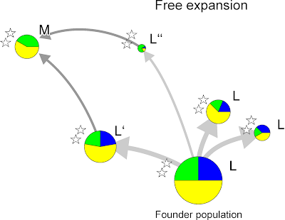
Why it's important to correlate genetic, linguistic and socio-cultural data. The doodle shows a simple free expansion model of a founder population with three genotypes (yellow, green, blue), a shared language (L) and two major cultural innovations (white stars). Because of drift and stochastic intra-population processes (size represent the size of the actively reproducing populace) the first expansion (light gray arrows) lead to 'tribes' that show already some variation. The smaller ones close to the founder population spoke still the same language, the ones further away used variants (dialects) of L (L', still close to L, L'', more distinct). Because of bootlenecks, geographic distance and differing levels of inbreeding (the smaller a population, the farther away from the source, the more likely are changes in genotype frequency), each population has a different genotype composition. The second expansion (mid-gray arrows) mixing two sources leads to a grandchild that evolved a new language M and lost the blue genotype. Because the cultural innovations are beneficial, we find them in the entire group. In extreme cases of genetic sorting and linguistic evolution, such shared cultural innovations may be the only evidence clearly linking all these populations.

Social-cultural character matrices

Correlating different sets of data and (cross-)exploring the signal in these data can be facilitated by creating suitable character matrices. In phylogenetics, we primarily use characters that underlie (ideally) neutral evolution, such as nucleotide sequences and their transcripts, amino-acid sequences. When using matrices scoring morphological traits, we relax the requirement of neutral evolution, but we are still scoring traits that are the product of biological evolution. However, we don't need to stop there, phylo-linguistics is an active field, even though languages involve different evolutionary constraints and processes than we meet in biology. Data-wise there are nonetheless many analogies, and phylogenetic methods seem to work fine.

So, why not also score socio-cultural traits in a character matrix? For instance, we can characterize cultures and populations by basic features including: the presence of agriculture, which crops were cultivated, which animals were domesticated, which technological advances were available, whether it was a stone-age, bronze-age, iron-age culture, etc. Linguistically, we could also develop matrices of local populations, with regional accents or dialects, etc.

Creating such a matrix should, of course, be informed by available objective information. As in the case of morphological matrices or non-biological matrices in general, we should not be concerned about character independence. We don't need to infer a phylogenetic tree from these matrices, as their purpose is just to sum up all available characteristics of a socio-cultural group.

Second phase: stabilization of differentiation pattern. While the close-by tribes are still in contact with the mother population, the most distant lost contact. As consequence the gene pools of the L/L'-speaking communities will become more similar, and new innovations acquired by the founder population (black star) are readily propagated within its cultural sphere. Re-migration from the larger M-speaking tribe to the struggling L''-speakers (small population with high inbreeding levels) lead to the extinction of the blue genotype in the latter and increased 'borrowing' of M-words and concepts.

Distance calculations

Pairwise distance matrices are most versatile for comparing data across different data sets.

First, any character matrix can be quickly transformed into a distance matrix, and the right distance transformation can handle any sort of data: qualitative, categorical data as well as quantitative, continuous data.

Second, the signal in any distance matrix can be quickly visualized using Neighbor-nets. This blog has a long list of posts showing Neighbor-nets based on all sorts of sociological data that don't follow any strict pattern of evolution, and are heavily biased by socio-cultural constraints (eg. bikability, breast sizes, German politics, gun legislation, happiness, professional poker, spare-time activities). We have even included celestial bodies.

Third, distance matrices can be tested for correlation as-is, without any prior inference, using simple statistics, such as the Pearson correlation coefficient. To give just one example from our own research: in Göker and Grimm (BMC Evol. Biol. 2008), the latter was used for testing the performance of character and distance transformations for cloned ITS data covering substantial intra-genomic diversity, by correlating the resulting individual-based distances with species-level morphological data matrices. (The internal transcribed spacers are multi-copy, nuclear-encoded, non-coding gene regions; in the simplest case each individual has two sets of copies, arrays, one inherited from the father, the other from the mothers, which may differ between but also within the individual.)

In the context of Racimo et al.'s paper, one could construct a genetic, a socio-cultural, a linguistic and a geographical matrix, determine the pairwise distances between what in phylogenetics are called OTUs (the operational taxonomic units), and test how well these data (or parts of it) correlate. The OTUs would be local human groups sharing the same culture (and, if known) language.

Alternatively, one can just map the scored socio-cultural traits onto trees based on genetic data or linguistics.

A new culture with its own language (Λ), genotype (red) and innovations (ruby-red pentagon) migrates close to the settling area of the L-people. Because of raids, genotypes and innovations from the the L-people get incorporated into the the Λ-culture.

How to get the same set of OTUs

The Göker & Grimm paper mentioned above tested several options for character and distance transformations, because we faced a similar problem to what researchers will face when trying to correlate socio-cultural data with genetic profiles of our ancestors: a different set of leaves (the OTUs). We were interested in phylogenetic relationships between individuals using data representing the genetic heterogeneity within these individuals.

Genetic studies of human (ancient or modern) DNA use data based from individuals, but socio-cultural and linguistic data can only be compiled at a (much) higher level: societies, or other groups of many individuals. In addition, these groups may also span a larger time frame. Since humans love to migrate, we are even more of a genetic mess than were the ITS data that we studied.

One potential alternative is to use the host-associate analysis framework of Göker & Grimm. Instead of using the individual genetic profiles (the associate data), one sums them across a socio-cultural unit (serving as host). The simplest method is to create a consensus of the data (in Göker & Grimm, we tested strict and modal consensuses). This produces sequences with a lot of ambiguity codes — genetic diversity within the population will be presented by intra-unit sequence polymorphism (IUSP). Standard distance and parsimony implementation do not deal with ambiguities, but the Maximum likelihood, as implemented in RAxML, does to some degree. A gapstop is the recoding of ambiguities as discrete states for phylogenetic analysis (tree and network inference) as done by Potts et al. (Syst. Biol. 2014 [PDF]) for 2ISPs ('twisps'), intra-individual site polymorphism. It can't hurt to try out whether this works for IUSPs, too.

Since humans (tribes, local groups) often differ in the frequency of certain genotypes, it would be straightforward to use these frequencies directly when putting up a host matrix. Instead of, for example, nucleotides or their ambiguity codes, the matrix would have the frequency of the different haplotypes. We can't infer trees from such a matrix (we need categorical data), but we can still calculate the distance matrix and infer a Neighbor-net.

The 'phylogenetic Bray-Curtis' (distance) transformation introduced in Göker & Grimm (2008) also keeps the information about within-host diversity when determining inter-host distances (see Reticulation at its best ...)


Transformations for genetic data from smaller to larger, more-inclusive units are implemented in the software package POFAD by Joli et al. (Methods in Ecology & Evolution, 2015. Their paper also provides a comparison of different methods, including the ones tested in Göker & Grimm (2008, also implemented in the tiny executables g2cef and pbc, compiled for any platform).

The process of assimilation. The Λ-people subdued the L-culture with the consequence that all innovations are shared in their influence sphere. Having a much smaller total population size, the language of the invaders is largely lost but the new common language L* still includes some Λ-elements (in a phylogenetic tree analysis, L* would be part of the L/M clade, using networks, L* would share edges with Λ in contrast to L and M). The L''/M-speaking remote population is re-integrated. The invaders' genotype (red) becomes part of the L-people's gene pool. Re-migration (forced or not) introduces L-genotypes into the original Λ-population. Only by comparing all available data, ideally covering more than one time period, we can deduce that the M-speakers represent an early isolated subpopulation of the L-people that was not affected by the Λ-invasion. With only the genetic data at hand, one may identify the M-speakers as one source and the Λ-tribe as another source for the L*-people, and infer that all L/M and Λ-tribes share a common origin (since the yellow genotype is found in both the M- and the original Λ-population).

Conclusion

It therefore seems to us that there is enormous potential for multi-disciplinary work, that truly combine organismal and socio-cultural evolution. We have provided a few practical suggestions here about how this might be done. We encourage you all to have try some of these ideas, to see where it leads us all.

Why the emperor has no clothes on – a thicket of trees

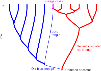
A critical question in phylogenetics, and this applies to both the detection and inference of reticulation, is: How much trust do we put in the inferred tree? A phylogenetic tree is just the simplest of all possible phylogenetic networks. Let's assume that there was some phylogenetic reticulation in the past (lineage mixing and crossing), then, in the best-case scenario, our inferred tree shows one of the intertwining pathways but misses the tangles, the crossroads.

An example of simple reticulate evolution: pink is the product of very recent lineage crossing between an early diverged (and otherwise lost) member of the blue lineage and the more recently, hence genetically more coherent, red lineage. Bold lines show the tree we would likely infer in such a situation.

In the worst case, summarizing data with substantially different signals will give us branching artifacts such as:

• terminal branches that are too long,
• too long internal branches with conspicuously low support (ie. BS << 100, PP < 1.0),
• artificial branches representing the least-conflicting solution for the conflicting data,
• low branch support in general.

See eg. the bear data we used as a real-world example for our Intertwining trees and networks paper (Schliep et al. 2017, open access).

Three possible trees for bears, (a), Y-chromosome, paternal, and (c), nuclear-encoded autosomal introns, biparentally inherited, are congruent but disagree with the maternal genealogy (b), based on the mitochondrial genes. When fusing all three data sets, we get a (low) supported sister relationship for Sloth and Sun bears (red clade), not supported by any of the three fused data set – a branching artifact.

Topological incongruence between gene trees and parental genealogies (as above) is commonly taken as evidence for reticulation. If one gene provides high support for taxon A as sister to B, and another gene has high support for B as sister to C, then B is likely the product of reticulation (eg. hybridization)

One simple possibility to put together a phylogenetic network is to summarize all of the trees in the form of a Consensus network, as shown next. (Technically this is a splits graph, it becomes a phylogenetic network as soon as we determine a root, which, here, would be at the edge leading to the Giant Panda.)

A strict Consensus network of the paternal, biparental, and maternal bear genealogies.
The numbers show the non-parametric bootstrap support for each (competing) split.

In this case, low support for a branch in a combined tree (the values on top) can result from strong conflict. For instance, the brownish splits, which are poorly supported using the combined data (BS = 21, 29), receive near unambiguous support from the mitochondrial genes, but are largely or entirely rejected by the Y-chromosome and nc-intron data. In the combined tree, this deep conflict is resolved by introducing the artificial red clade, with similarly low support: the signal in the data is ambiguous and they support splits between equally possible alternatives.

We know lineage crossing took place in bears (the mitochondrial and Y-chromosome tree are very much in conflict). However, does the above mean that earliest bear-ish creatures hybridized, too? Note that the conflict is associated with a short-branched part of the graph, where apparently little evolution happened. Fast ancient radiations usually come with incomplete lineage sorting and diffuse signals. The only data set producing longer roots, but with notably lower support, are the biparentally inherited introns.

We are closing in our own tail and have to ask again: Is this low support in the autosomal intron tree due to internal conflict, (sets of) introns preferring different topologies, supporting an ancient mixing hypothesis, or just reflecting lack of resolution? Check out the original paper by Kutschera et al. (2014, Mol. Biol. Evol. 31: 2004–2017), and make up your own mind.

On to the angiosperms

In my last post, I exemplified what Walker et al. (PeerJ, 2019) found in their angiosperm study: when we look at a plastome tree we are not looking at a summary of all gene trees but instead at a topology forced by very few of the genes in the chloroplast genome, such as the matK. We also have seen that one misplaced sequence (outgroup Podocarpus-matK) doesn't affect at all the combined analysis — it didn't even reduce the ingroup - outgroup split support. Also, I noted that the low-supported part of the combined tree goes hand in hand with lack of decisive signal from the matK.

It's time to take a look at what the other genes in this example data set come up with.

The eight gene trees. Terminal subtrees collapsed. Scales fit to size, scale bar = 0.1 expected substitutions per site. Upper left, matK tree which is very similar to the combined tree using all gene regions (cp = chloroplast, mt = mitochondrial, nc = nuclear genes). Note the low performance of the mt genes.

One thing is obvious: for most genes (except the nuclear-encoded rRNA genes) including the outgroup taxa adds little ingroup information of use — they are just too distant to any of the ingroup taxa. Outgroup rooting is tricky for angiosperms. Outgroup taxa will always be attracted to the ingroup taxon that is the least similar to any other part of the ingroup: Amborella in this case.

Generally, all of the ANA-grade water plants are genetically distinct and topologically isolated; any outgroup-inferred root must be placed in this part of the tree (all other living seed plants are very distant relatives of angiosperms looking back at, at least, ~250 million years of independent evolution, see eg. Age of Angiosperms... and What is an angiosperm pt. 2). The relatively conserved plastid rbcL and mitochondrial matR prefer an Amborella-Nympheales clade as sister to all other angiosperms, while the more divergent atpB, plastid, nad5, mitochondrial, and 25S, nuclear, prefer the Amborella-root — this is a direct indication for ingroup-outgroup long-branch attraction. Any other placement of the outgroup subtree within the ingroup would necessarily decrease the likelihood of the tree (but note the position of the root in the 18S tree, lower-left the tree based on the most-conserved, evolution-constrained gene in our sample; see also All solved a decade ago..., fig. 4A).

We can look at these trees with the strict consensus network, using uninformed edge lengths— that is, the network counterpart to the strict consensus cladograms still common in plant phylogenetic literature.

This is a nice piece of computer-art, but is scientifically quite useless (the boxiness and general graph structure is, however, reminiscent of strict consensus networks of most-parsimonious tree samples inferred for extinct animals, one example, and plants).

We can add some discriminatory information by counting how often each split occurs in the set of gene trees.

Same set of tree, different way of summarizing it. Note how the main clades emerge: one or two genes may have misplaced the one or other OTU but the others get it right.

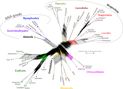
Alternatively, we can average the actual tree branch lengths to inform the edge length of the consensus network.

The light green, sand-colored, light brown and dark olive (clockwise) splits are likely branching artifacts. The light blue split is the one that supports the ANA-grade when the (combined) tree is rooted with the very distant outgroups.

A pretty little thicket of trees. Some agreement is found towards the leaves, but even here we have conflict among the gene trees. In some trees, there are long branches grouping non-related OTUs, obvious tree inference artifacts. The general rule is that the deeper we go (ie. the farther back in time), the messier it gets. Adding to this is that, irrespective of which gene is used, some OTUs are much closer to the hypothetical common ancestor (of Mesangiosperms, ie. all but ANA grade) than others – in the eudicots, the least-evolved taxa are Platanus (very old tree genus) and Euptelea (the basalmost Ranunculales); in the Magnoliales, the only angiosperm clade that lacks synapomorphies, it's Magnolia and Liriodendron (again, very old and primitive tree genera). Darwin's Abominable Mystery, the sudden appearance and quick dominance of angiosperms, resulted in an abominable chaos of gene trees and signals. How can they possibly converge to a single tree with amply high support along most branches?

The combined tree from the first post.

When compared to the bears, the answer may well be: because there has been very little to no reticulation between these lineages. Our thicket may be not a forest of trees but just a poorly trimmed, wildly overgrown bush. They genes share the same history, but when being analyzed one-by-one, each of their trees get some aspects right, and some others (severely) wrong. Misplacing one OTU (e.g. the light green, dark olive, sand-colored and dark yellow splits in the averaged Consensus network) may have further topological effects; it didn't matter for the matK gene, because we misplaced only one very alien OTU in a data set that otherwise is hardly affected by adding or removing OTUs.

I argue here that, if there had been substantial reticulation messing up the signal of contemporary lineages and reflecting decoupled histories (like in the case of bears), we would expect at least some (artificial) branching patterns with low support in the combined tree, as well. This would also be the case looking at the gene-tree consensus networks, not only in the deepest parts but also closer to the leaves.

We will be explore this alternative hypothesis in the next (and final) post of this mini-series.