Why are splits graphs still called phylogenetic networks?

This is an issue that has long concerned me, and which I think causes a lot of confusion among biologists. A phylogenetic tree is usually a clear concept — to a biologist, it is a diagram that displays a hypothesis of evolutionary history. The expectation, then, is that a phylogenetic network does the same thing for reticulate evolutionary histories. However, this is not true of splits graphs; and so there is potential confusion.

Mathematically, of course, a phylogenetic tree is a directed acyclic line graph. It is usually constructed, in practice, by first producing an undirected graph based on some pattern-analysis procedure, and then nominating one of the nodes or edges as the root (say, by specifying an outgroup). So, the mathematics is not really connected to the biological interpretation. To a mathematician, the tree is a set of nodes connected by directed edges, and the nodes could represent anything at all, as could the edges. It is the biologist who artificially imposes the idea that the nodes represent real historical organisms connected by the flow of evolution — ancestors connected to descendants by evolutionary events.

A phylogenetic network should logically be a generalization of this idea of a phylogenetic tree, adding the possibility of evolutionary relationships due to gene flow, in addition to the ancestor-descendant relationships. This can be done, but it is only partly done by splits graphs.

That is, a splits graph generalizes the idea of an undirected line graph (an unrooted tree), but not a directed acyclic graph (a rooted tree). It follows the same logic of using a pattern-analysis procedure to produce an undirected graph, although the graph can have reticulations, and thus is a network rather than necessarily being a bifurcating tree. However, it is not straightforward to specify a root in a way that will turn this into an acyclic graph. So, in general it does not represent a phylogeny.

Indeed, splits graphs are simply one form of multivariate pattern analysis, along with clustering and ordination techniques, which are familiar as data-display methods in phenetics (see Morrison D.A. 2014. Phylogenetic networks — a new form of multivariate data summary for data mining and exploratory data analysis. Wiley Interdisciplinary Reviews: Data Mining and Knowledge Discovery 4: 296-312). In this sense, it makes no difference whatsoever what the data represent — they can be data used for phylogenetics, or they could be any other form of multivariate data. Indeed, this point is illustrated in many of the posts in this blog, which can be accessed in the Analyses page.

So, unlike unrooted trees, unrooted splits graphs are not a route to producing a phylogenetic diagram. Mind you, they are a very useful form of multivariate data analysis in their own right, and I value them highly as a form of exploratory data analysis. But that doesn't make them phylogenetic networks in the biological sense.

So, isn't it about time we stopped calling splits graphs "phylogenetic networks"? They aren't, to a biologist, so why call them that?

Tree Alignment Graphs and data-display networks

Data-display networks are a means of visualizing complex patterns in multivariate data. One particular use is for displaying the patterns in a set of trees. For example, Consensus Networks and SuperNetworks are splits graphs that display the patterns common to some specified subset of a collection of trees (eg. a set of equally optimal trees, or a set of trees sampled by a bayesian or bootstrap analysis). Alternatively, Parsimony Networks try to simultaneously display all of the trees in a collection of most-parsimonious trees for a single dataset.

Another display method for multiple trees is what has been called a Cloudogram (see the post Cloudograms and data-display networks). These superimpose the set of all trees arising from an analysis, so that dark areas in such a diagram will be those parts where many of the trees agree on the topology, while lighter areas will indicate disagreement.

Yet another method for combining trees into a graph while retaining all of the original information from the source trees is the Tree Alignment Graph (TAG), an idea introduced by Stephen A. Smith, Joseph W. Brown and Cody E. Hinchliff (2013. Analyzing and synthesizing phylogenies using tree alignment graphs. PLoS Computational Biology 9: e1003223).

The authors note:

These methods address the problem of identifying common nodes and edges across sets of phylogenetic trees and constructing a data structure that efficiently contains this information while retaining original source information ... Mapping trees into a TAG exploits the fact that rooted phylogenetic trees are in fact a specific type of graph: they are directed, acyclic, and require that each node has, at most, one parent. By relaxing these requirements, we can combine multiple trees into a common graph, while minimizing changes to the semantic interpretations of nodes and edges in the trees. Because they contain nodes and edges directly analogous to those from their source trees, TAGs have the desirable quality of retaining the full identifiability of the original source trees they contain. Additionally, because they are not restricted to the bifurcating model of evolution, TAGs may represent conflict among source trees as reticulations in the graph.

The basic principal is illustrated in the first figure (about). Internal nodes represent collections of terminal nodes, and arcs (directed edges) represent their relationships. Nodes and arcs are added to the growing TAG, each of which represents one relationship shown in one of the original trees. TAG A in the figure shows the result of combining the black, blue and orange trees, while TAG B shows the result of then adding the gray and green trees to TAG A (the arcs are colour-coded). The resulting TAG is thus a database of all of the original information, which can then be queried in any way to provide summaries of the data. In particular, standard network summaries can be used, such as node degree, which will highlight parts of the TAG with interesting characteristics.

The authors provide two empirical examples of applications. The one shown here involves 100 bootstrap trees for 640 species representing the majority of known lineages from the Angiosperm Tree of Life dataset (chloroplast, mitochondrial, and ribosomal data). The TAG is shown lightly in the background. Superimposed on this, the nodes are coloured to represent the effective number of parent nodes, and their size represents node bootstrap support. Highly supported nodes with a low number of effective parents (large blue nodes) are frequently recovered and confidently placed in the source trees, while highly supported nodes with a low number of effective parents (large and pink or orange) are frequently resolved in the source trees but their placement varies among bootstrap replicates. So, the three largest problem areas as illustrated in the TAG correspond to the Malpighiales, Lamiales and Ericales.

For comparison, a NeighborNet analysis of the same data is shown in the blog post When is there support for a large phylogeny? This simply shows an unresolved blob.

Phylogenetic networks and "evolutionary networks"

Complex networks are found in all parts of biology, graphically representing biological patterns and, if they are directed networks, also their causal processes. Directed networks are currently used to model various aspects of biological systems, such as gene regulation, protein interactions, metabolic pathways, ecological interactions, and evolutionary histories.

Two types of networks can be distinguished, and this distinction seems to me to be very important. Most networks are what might be called observed networks, in the sense that the nodes and edges represent empirical observations. For example, a food web consists of nodes representing animals with connecting edges representing who eats whom. Similarly, in a gene regulation network the genes (nodes) are connected by edges showing which genes affect the functioning of which other genes. In all cases, the presence of the nodes and edges in the graph is based on experimental data. These are collectively called interaction networks or regulation networks.

However, when studying historical patterns and processes not all of the nodes and edges can be observed. So, instead, they are inferred as part of the data-analysis procedure. That is, we infer the patterns as well as the processes; and we can call these inferred networks. In this case, the empirical data may consist solely of the leaf nodes, and we infer the other nodes plus all of the edges. For example, every person has two parents, and even if we do not observe those parents we can infer their existence with confidence, as we also can for the grandparents, and so on back through time with a continuous series of ancestors. Alternatively, we may also observe some of the internal nodes of the network, such as when we do record the parents and grandparents because they are contemporaneous (ie. their generations overlap). This type of pattern can be represented as a genealogical network, when referring to individual organisms, or a phylogenetic network when referring to groups (populations, species, or larger taxonomic groups).

What, then, are the things often referred to as "evolutionary networks" but which are clearly not phylogenetic networks? They are of the first type, the interaction networks. In an evolutionary network the observed nodes are directly connected to each other to represent some aspect of evolution. This aspect may have some component of phylogeny to it, but there is more to the study of evolution than solely phylogenetic history.

For example, directed LGT (dLGT) networks connect nodes representing contemporary organisms with edges that represent inferred lateral gene transfer. That is, the evolutionary networks show gene sharing. This is obviously related to the phylogeny of the organisms, but the network does not display the phylogeny itself. This first example (from Ovidiu Popa, Einat Hazkani-Covo, Giddy Landan, William Martin, Tal Dagan. 2011. Directed networks reveal genomic barriers and DNA repair bypasses to lateral gene transfer among prokaryotes. Genome Research 21: 599-609) shows "32,028 polarized lateral recipient–donor protein-coding gene transfer events" inferred from "the completely sequenced genomes of 657 prokaryote species".

The concept of a gene-sharing network as an evolutionary network has also been applied to viruses and their relatives, for example, as shown by this next diagram (from Natalya Yutin, Didier Raoult, Eugene V Koonin. 2013. Virophages, polintons, and transpovirons: a complex evolutionary network of diverse selfish genetic elements with different reproduction strategies. Virology Journal 10: 158).

The question, then, is what to make of diagrams that combine both a phylogenetic tree and this type of evolutionary network, such as is done in the Minimal Lateral Network. This next example is from linguistics rather than biology (from Johann-Mattis List, Shijulal Nelson-Sathi, Hans Geisler, William Martin. 2013. Networks of lexical borrowing and lateral gene transfer in language and genome evolution. Bioessays 36: 141-150), and it superimposes the sharing network and the phylogenetic tree. (For a discussion in the context of LGT, see also Tal Dagan. 2011. Phylogenomic networks. Trends in Microbiology 19: 483-491).

In this diagram, the tree explicitly represents the phylogenetic history of the languages while the evolutionary network represents possible borrowings of words, with thicker lines representing more borrowed words. Clearly, the network also contains phylogenetic information of some sort. For example, the connection of the root of the Romance languages to English reflects the conquest of Britain by the French-speaking Normans, which modified the Old-German heritage of Old English. However, the diagram as a whole is a hybrid, rather than being a coherent phylogenetic network in the simplest sense (ie. a reticulation network).

To see this clearly, note that the phylogenetic tree is not fully resolved and that the evolutionary network does suggest possible resolutions for several of polychotomies, such as the relationship of Armenian and Greek, the relationship of Albanian to the Romance languages, and the relationship of the Gaelic languages to the Romance languages. So, in some cases the evolutionary network helps resolve the phylogenetic tree rather than forming a reticulating network.

It would be possible to derive a phylogenetic network from this minimal lateral network, but as it stands it is a combination of a phylogenetic tree and a so-called evolutionary network.

Monophyletic groups in networks

I have noted before that taxonomic groups that are represented in any tree-like parts of a phylogeny can be considered to be monophyletic, but those that consist of hybrids cannot, unless we hypothesize a single hybrid origin for each group (How should we treat hybrids in a taxonomic scheme?). This issue arises from the concept that monophyletic groups must share an exclusive Most Recent Common Ancestor (MRCA), and this concept is not straightforward for a network compared to a tree.

This topic has been tackled mathematically a couple of times (see Huson and Rupp 2008; Fischer and Huson 2010), resulting in the recognition that for a network there are three main types of MRCA: conservative MRCA (or stable MRCA), Lowest Common Ancestor (or minimal common ancestor), and Fuzzy MRCA (see Networks and most recent common ancestors). These have definitions based on the Least Lower Bound and Greatest Lower Bound of mathematical lattices.

Unfortunately, there has been very little discussion of the topic in the biological literature. However, recently Wheeler (2013) has made a start. There is no reference to the mathematical work on MRCAs, but he considers what to do about the concepts of monophyly, paraphyly and polyphyly with respect to networks.

Basically, he suggests three new types of phyletic group: periphyletic, epiphyletic, and anaphyletic. He provides algorithmic definitions of these groups, relating them to the previous algorithmic definitions of monophyly, paraphyly and polyphyly. These new types concern groups that are monophyletic on a tree, but have additional gains or losses of members from network edges — that is, they lie somewhere between monophyletic and paraphyletic.

For example, an epiphyletic group would be one that is otherwise monophyletic but also contains one or more hybrids that have one of their parents from outside the group, while a periphyletic group would be monophyletic but has contributed as a parent to at least one hybrid outside the group. An anaphyletic group would have done both of these things. For clarification, Wheeler provides the following empirical example, based on Indo-European languages (where English is recognized as a "hybrid" of Germanic and Romance languages).

Reproduced from Wheeler (2013).

In terms of MRCA, it seems to me that all three new group types use the Lowest Common Ancestor model, which is the shared ancestor that is furthest from the root along any path (ie. the LCA is not an ancestor of any other common ancestor of the taxa concerned). However, this is only clear when we consider hybrids, in which the two (or more) parents contribute equally to the hybrid offspring. When dealing with introgression or horizontal gene transfer, where the parentage is unequal, then we approach the Fuzzy MRCA model, in which only a specified proportion of the paths (representing some proportion of the genomes) needs to be accommodated by the MRCA, thus keeping the MRCA close to the main collection of descendants.

What is not yet clear is whether we would want to recognize any of these new group types in a taxonomic scheme. I guess that this is something that the PhyloCode will have to think about, since it is based strictly on clades (although they are allowed to overlap).

References

Fischer J, Huson DH (2010) New common ancestor problems in trees and directed acyclic graphs. Information Processing Letters 110: 331–335.

Huson DH, Rupp R (2008) Summarizing multiple gene trees using cluster networks. Lecture Notes in Bioinformatics 5251: 296–305.

Wheeler WC (2013) Phyletic groups on networks. Cladistics (online early).
Wheeler WC (2014) Phyletic groups on networks. Cladistics 40: 447-­451.

Should phylogenetic modelling proceed from simple to complex or vice versa?

In statistical model testing, models can be tested by starting with the simplest model and progressively adding model complexity until the desired level of model fit is achieved. Alternatively, one can start with the most complex model and progressively delete unnecessary components while maintaining the desired level of model fit. The first approach is constructive, in the sense that the model is constructed piece by piece (stepwise addition), while the second approach is reductive, in the sense that the full model is pared down to its simplest form (stepwise deletion).

This distinction in approaches to modelling is relevant to the difference between using trees and networks as phylogenetic models.

At the moment, the most common approach to phylogenetic analysis is the constructive one. One starts with the simplest model, a bifurcating tree, and assesses the degree to which it fits the data. If the fit is poor, as it often is with multi-gene data, especially if the gene data are concatenated, then complexity is added. For example, one might include incomplete lineage sorting (ILS) in the model, which allows the different genes to fit different trees, while still maintaing the need for a single dichotomous species tree. Alternatively, one might consider gene duplication-loss as a possible addition to the model, which is another major source of incompatibility between multi-gene data and a single species tree. Only if these additional complexities also fail to attain the desired degree of fit does one consider adding components of reticulate evolution to the model, such as hybridization or horizontal gene transfer (HGT).

The reductive (or simplification) approach, however, proceeds the other way. A general network model is used as the starting point. The various components of this model would include a dichotomous tree as a special case, along with ILS, duplication-loss, hybridization, and HGT as individual components. These special cases are evaluated simultaneously, and each one is dropped if it is contributing nothing worthwhile to the model fit. The final model consists of the simplest combination of components that still maintains the specified fit of data and model; this may indeed be a simple tree.

The main advantage of the latter approach is that all of the components of the model are evaluated simultaneously, so that their potential interactions can be quantitatively assessed. Components are dropped from the model only if they contribute nothing to the model, either independently or in synergy with the other components. That is, they are dropped only if they can be shown to be redundant.

This does not happen with the constructive approach to modelling. Here, the components are evaluated in some specified order, and components that are later in the order will not be evaluated unless the earlier components prove to be inadequate. These later components are thus potentially excluded from statistical consideration. This means that their possible contribution to biological explanation may never be quantitatively assessed.

So, in practice, evolutionary reticulation is considered to be a "last resort" in current phylogenetic analyses. It is considered as a possible biological explanation only if all else has already failed.

This philosophy seems to be as much a historical artifact as anything else. The first phylogenetic diagrams (by Buffon and Duchesne) were networks not trees, but they were replaced a century later by the tree model suggested by Darwin; and the tree has retained its primacy since that time. This leads naturally to the constructive approach to modelling, which is so prevalent in the current literature.

However, there is no necessary statistical superiority of the constructive approach to modelling. Indeed, statisticians seem to consider forward and backward selection of model components to be essentially equivalent, although they may lead to different models for any given dataset. The most commonly specified advantage of the constructive approach to modelling is that it is likely to avoid possible problems arising from having too many components in the model.

Nevertheless, the reductive approach has the distinct advantage of simultaneously evaluating all possible special cases of a network, and thus does not exclude any possible biological explanation that might apply to the observed data. This may provide more biological insight than does the construcive approach to phylogenetic modelling.

Networks and most recent common ancestors

The interpretation of an evolutionary network is confounded by the fact that descendants of reticulation nodes have complex ancestry. Therefore, the concept of a Most Recent Common Ancestor (MRCA) is not as straightforward as it is for a tree, as there may be multiple paths from any one descendant back to its ancestors. This creates several possible interpretations of what we might mean by a MRCA.

Figure 1 illustrates the calculation of the MRCA in a tree of five taxa (A-E), showing the MRCA of taxa C and D. We simply trace each of the descendant taxa backward along the branches towards the root, and the ancestral node where all of these traces first intersect is the MRCA of those taxa.

Figure 1.

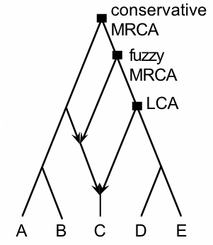
Figure 2 illustrates a more complex history, involving two hybridization events. The incoming branches to the reticulation nodes have arrows, for emphasis. The figure also recognizes several possible interpretations of the MRCA of taxa C and D (see Huson and Rupp 2008; Fischer and Huson 2010).

A conservative definition of the MRCA (or a stable MRCA) is the intersection of all paths from the descendants to the root, so that any reticulation pushes the MRCA back towards the root. In this example it pushes the MRCA all the way to the root. Alternatively, we could define the Lowest Common Ancestor (or the minimal common ancestor) as the shared ancestor that is furthest from the root along any path. That is, the LCA is not an ancestor of any other common ancestor of the taxa concerned.

Figure 2.

In the mathematical terminology of lattices, which can have an algebraic or order theoretic definition, the Conservative MRCA is called the Least Lower Bound (LLB) and the LCA is called the Greatest Lower Bound (GLB).

We could also have a biological compromise between these two mathematical concepts and recognize a Fuzzy MRCA, in which only a specified proportion of the paths (representing some proportion of the genomes) needs to be accommodated by the MRCA, thus keeping the MRCA close to the main collection of descendants (Fischer and Huson 2010). In this example, the Fuzzy MRCA represents 75% of the genome of taxon C and 100% of the genome of taxon D. (The Conservative MRCA represents 100% for both taxa, by definition; and in this example the LCA represents 50% of the genome of taxon C and 100% of the genome of taxon D.)

Figure 3.

However, neither the Fuzzy MRCA nor the LCA is necessarily unique, although the Conservative MRCA will always be unique. Figure 3 shows an example where there are two independent LCAs of taxa C and D. Neither of these LCAs is an ancestor of the other, as required by the definition, and so they are both equal candidates as LCA. Each one represents 50% of the genome for both taxa C and D.

In terms of a lattice, Figure 2 is called a lower semi-lattice (or meet semi-lattice), because every pair of nodes has only one GLB, whereas Figure 3 is not a semi-lattice, because at least one node pair has more than one GLB.

This leads to the biological question of how we are best to interpret the MRCA in situations such as that represented by Figure 3. This is a question that does not yet seem to have been addressed by biologists. Figure 3 does not represent an impossible evolutionary history, although it may be an unusual one because one lineage hybridizes with another lineage twice, presumably at different times.

The lack of a unique LCA is clearly problematic, as it almost defeats the purpose of the concept of a MRCA. It would certainly make life easier if we could restrict evolutionary networks to the class of lower semi-lattices.

An alternative is to restrict the MRCA concept to the Conservative MRCA. However, it is easy to imagine situations where this pushes the MRCA so far towards the root of the network as to be uninformative, especially in cases involving horizontal gene transfer, which can occur between widely separated evolutionary groups. If we insist that a eukaryote MRCA represent 100% of the genome, and we include non-nuclear genomes in the calculation, then the Conservative MRCA creates an extreme theoretical problem.

A Fuzzy MRCA may be the best compromise between these two extremes, although there are obvious practical issues for obtaining agreement on how much of the genome history is to be discounted from the MRCA.

References

Fischer J., Huson D.H. (2010) New common ancestor problems in trees and directed acyclic graphs. Information Processing Letters 110: 331–335.

Huson D.H., Rupp R. (2008) Summarizing multiple gene trees using cluster networks. Lecture Notes in Bioinformatics 5251: 296–305.

Are mathematical constraints biologically realistic?

Mathematicians and other computational scientists have produced their own definitions of phylogenetic networks, independently of biologists. For the evolutionary type of phylogenetic network, the definition usually looks something like this:

A phylogenetic network is a rooted, directed graph (consisting of nodes, plus edges that connect each parent node to its child nodes) such that:
(1) There is exactly one node having indegree 0, the root
        - all other nodes have indegree 1 or 2
(2) All nodes with indegree 1 have outdegree 2 or 0
        - nodes with outdegree 2 are tree nodes
        - nodes with outdegree 0 are leaves, distinctly labelled
(3) The root has outdegree 2, and
(4) Nodes with indegree 2 have outdegree 1, called reticulation nodes.

An obvious question of interest is how (or whether?) this definition connects to what biologists have in mind when they use the term "phylogenetic network". Clearly, this definition places considerable restrictions on the networks that will be inferred by any mathematical algorithm, which in turn affects their use as models for biological inference.

The first thing to note is that unrooted networks are excluded, because the graph is directed. Thus, many (if not most) of the phylogenetic networks that have appeared in the literature are excluded from the discussion. Furthermore, a tree is considered to have all internal nodes with indegree 1 and outdegree 2 (i.e. no reticulation nodes), and we know this to be biologically unrealistic, in general. (Otherwise, this blog would be redundant!)

Biologically, the other parts of the definition imply:
One node of indegree 0
- the network has no previous ancestry that is to be inferred
Nodes with outdegree 0 are labelled
- observed (contemporary) taxa occur only at the leaves
All nodes with indegree 2 have outdegree 1
- reticulation and speciation cannot occur simultaneously
No nodes with indegree >2
- reticulation events cannot involve input from more than 2 parents simultaneously
No nodes with outdegree >2
- speciation involves only two children at a time.

These do not appear to be onerous biological restrictions. Indeed, he first two have been standard characteristics of tree-building for several decades. The other three are also logical extensions of  the restrictions that have previously been placed on trees. However, phylogenetic history is unlikely to have been as simple as implied by these features. Thus, biologists will need to keep a careful eye on whether the simplifications are affecting the networks inferred for their particular group of organisms.

Other restrictions

In addition to the restrictions created by the definition, other topological restrictions have been used to make the mathematical inference algorithms computationally tractable. Thus, only certain sub-families of possible networks are considered by most of the computer programs. These include:

• tree-child network, tree-sibling network
• level-k network, galled tree
• binary input trees for hybridization and HGT networks
• binary characters for recombination networks.

These restrictions may be unrelated to each other; so, we can consider them separately.

Tree-child, Tree-sibling

In a tree-child network, every internal node has at least one child node that is a tree node
- ie. a reticulation event cannot be followed immediately by another reticulation event
In a tree-sibling network, every reticulation node has at least one sibling node that is a tree node
- ie. a parent cannot be directly involved in two separate reticulation events
Note that every tree-child network will also be a tree-sibling network, but not vice versa.

Algorithmically, these two restrictions may involve the addition of extra tree nodes to an inferred network, in order to satisfy the restrictions. Biologically, the question is whether real networks are this simple. Arenas et al. (2008) simulated data under the coalescent with recombination, and found that even at small recombination rates most of the networks produced were already more complex than a tree-sibling network. On the other hand, Arenas et al. (2010) analyzed real population-level data from the PopSet and Polymorphix databases using the TCS program, and found that >98% the resulting networks could be characterized as tree-sibling. So, there is cause for optimism, in the sense that the "optimum" networks algorithmically are not necessarily complex, at least for closely related organisms (ie. within species).

Level-k network, Galled tree

A network has level k if each tangled part of the network (ie. each biconnected component) contains at most k reticulation nodes (see this previous post). This is a generalization of the older notion of galled trees, in which reticulation cycles do not overlap (ie. do not share edges or nodes), as galled trees are level-1 networks. Level-k networks can also be seen as a generalization of networks with k reticulation nodes, although there may be a difference between a network with minimum level and one with a minimum number of reticulations.

Algorithmically, these restrictions have been used to guide the search for (or choice of) the "optimal" inferred network. Biologically, these notions do not seem to have been investigated, but basically they restrict how complex inferred reticulation histories can be. In particular, they restrict the complexity of any given subset of each network. It has been noted that optimizing k can easily lead to networks that look biologically unrealistic (Huson et al. 2011).

Binary input

The requirements for binary input trees and binary characters are restrictions that have been applied in the past, because they greatly reduce the complexity of the input to the network algorithms, but they are now being relaxed. Effectively, the restrictions are to fully dichotomous trees and SNP characters. These are not unusual restrictions in evolutionary analysis, but they are obviously unrealistic.

As I noted in an earlier blog post, non-binary data often reflect uncertainty in the input, rather than a strictly bifurcating history, and this is not taken into account in the network inference if the input is restricted to a binary state. In particular, it may be unnecessarily hard to construct a network (because not all of the data signals relate to reticulation), and the resulting networks may have far too many reticulation nodes.

Conclusion

It is still an open question about the extent to which we can use these topologically restricted families of mathematical networks as a basis for reconstructing biological histories. Clearly, much more work is needed to understand the connections between the mathematical restrictions and the requirements of biological modelling.

References

M. Arenas, M. Patricio, D. Posada, G. Valiente (2010) Characterization of phylogenetic networks with NetTest. BMC Bioinformatics 11: 268.

M. Arenas, G. Valiente, D. Posada (2008) Characterization of reticulate networks based on the coalescent with recombination. Molecular Biology and Evolution 25: 2517-2520.

D. H. Huson, R. Rupp, C. Scornavacca (2011) Phylogenetic Networks: Concepts, Algorithms and Applications. Cambridge University Press.

Time inconsistency in evolutionary networks

The temporal ordering of the nodes (and branches) is usually treated as an important feature in an evolutionary network of biological organisms, because the order must be time consistent (Baroni et al. 2004, 2006; Moret et al. 2004). That is, for reticulation events the "horizontal" gene flow can only occur between species that are contemporaries. So, speciation events occur successively but reticulation events occur instantaneously (Sang and Zhong 2000).

For example, it would be unrealistic to hypothesize either a hybridization or a horizontal gene transfer event between a species and one of its own ancestors. Furthermore, each reticulation event must not only be consistent on its own but must be consistent in relation to all of the other events.

Mathematically, inconsistency creates directed pseudo-cycles in the network graph, so that it is not acyclic, as required for an evolutionary history (see previous blog post). Time consistency is thus seen as a useful means of validating a network as a potential biological history, and can even be used as a criterion for choosing among otherwise equally optimal networks.

However, evolutionary analysis is not applied only to biological organisms. It has also been applied to the study of languages (Atkinson & Gray 2005) and to cultural objects (Collard et al. 2006). Indeed, Darwin himself recognized early on that it would be important to show that language (a characteristic solely of humans) had a natural origin and that it develops in a genealogical fashion (ie. it has a pedigree).

Thus, both language and cultural objects have an historical component that can be studied, and both can fit into an evolutionary framework of variation + transmission + selection (Dagg 2011). Moreover, the evolutionary history also consists of both vertical and horizontal transmission. This means that the same data-analysis techniques can potentially be applied to biology, language and culture (Heggarty et al. 2010; Gray et al. 2010).

The issue that I wish to raise here is that time consistency is not a requirement of the evolution of either language or cultural objects, the way that it is for biological organisms. Organisms store the information (that is vertically and horizontally transmitted) in genes that they carry with them, which is what restricts reticulation to occurring only between contemporaries. However, language and culture store their "information" externally, either in the minds of people or in permanent or semi-permanent records (either written or pictorial). Thus, the information available for horizontal transmission can come from the distant past, as well as from the present. *

It is important to note that for language and culture the biological ideas of vertical and horizontal transmission of genetic information need modification (Cavalli-Sforza and Feldman 1981). Vertical (or descending) transmission still involves faithful copying of the information (with perhaps some losses or minor modifications). Lateral transfer, however, can be either horizontal transmission (between contemporary generations) or oblique transmission (between different generations), and it is the latter that allows time-travel of information.

Lateral transfer in this context may be a form of hybridization, in which new concepts are added from elsewhere (eg. synonymous words), but is likely to be a form of HGT in which concepts are simply replaced with something from elsewhere (eg. a new word effectively replaces an old word). Recombination, in which concepts are mutually exchanged, may be rather rare.

As an illustration, Dagg (2011) provides some interesting examples of lateral transfer in the parts of mouse traps. For example, he notes that: "Torsion power may have been transmitted laterally from Egyptian torsion traps to prefabricated dead-fall traps." These traps need not be contemporaneous, because the ideas being transferred may be from pictures or descriptions of old traps rather than from concurrently existing traps. (Joachim Dagg also has a couple of blog posts where he further discusses the evolution of mouse traps: post 1 —  post 2.)

As an alternative example, Johnson et al. (1989) provide an evolutionary network showing the history of the various software (mostly) and hardware components of the revolutionary Xerox 8010 "Star" Information System (ie. computer), introduced in April 1981. Note that almost all of the lateral transfer events (single arrows; mostly hybridization) are time inconsistent. To quote the authors: "Although Star was conceived as a product in 1975 and was released in 1981, many of the ideas that went into it were born in projects dating back over three decades."

Fig. 8 – How systems influenced later systems.
This graph summarizes how various systems related to Star have influenced one another over the years. Time progresses downwards. Double arrows indicate direct successors (i.e., follow-on versions). Many "influence arrows" are due to key designers changing jobs or applying concepts from their graduate research to products.

The implications of time-travelling laterally transferred information for network construction methods may be unfortunate, in the sense that evolutionary networks in biology may be quite different from those for language and culture, with the latter pair requiring somewhat different methods. At a minimum, the requirements for choosing among alternative networks will be different.

A quick look at the current literature involving network analysis of languages and cultural artifacts shows an almost universal use of unrooted graphs, most often a Neighbor-Net, Reduced-Median or Median-Joining network. Such networks cannot directly represent evolutionary history because there is no time direction in the graph. This type of analysis thus neatly side-steps the issue of representing time-travelling information in an evolutionary diagram; and it suggests that social scientists have not yet considered the consequences of the potential lack of time consistency in their data.

* Footnote: I suppose that I should be precise, and note that a modern gene bank does allow genetic information to time travel, as well.

References

Atkinson QD, Gray RD (2005) Curious parallels and curious connections — phylogenetic thinking in biology and historical linguistics. Systematic Biology 54: 513-526.

Baroni M, Semple C, Steel M (2004) A framework for representing reticulate evolution. Annals of Combinatorics 8: 391–408.

Baroni M, Semple C, Steel M (2006) Hybrids in real time. Systematic Biology 55: 46–56.

Cavalli-Sforza LL, Feldman MW (1981) Cultural Transmission and Evolution. Princeton University Press, Princeton.

Collard M, Shennan SJ, Tehrani JJ (2006) Branching, blending, and the evolution of cultural similarities and differences among human populations. Evolution and Human Behavior 27: 169–184.

Dagg JL (2011) Exploring mouse trap history. Evoluton: Education and Outreach 4: 397–414.

Gray RD, Bryant D, Greenhill SJ (2010) On the shape and fabric of human history. Philosophical Transactions of the Royal Society of London series B 365: 3923-3933.

Heggarty P, Maguire W, McMahon A (2010) Splits or waves? Trees or webs? How divergence measures and network analysis can unravel language histories. Philosophical Transactions of the Royal Society of London series B 365: 3829-3843.

Johnson J, Roberts TL, Verplank W, Smith DC, Irby C, Beard M, Mackey K (1989) The Xerox "Star": a retrospective. IEEE Computer 22: 11-29.

Moret BME, Nakhleh L, Warnow T, Linder CR, Tholse A, Padolina A, Sun J, Timme R (2004) Phylogenetic networks: modeling, reconstructibility, and accuracy. IEEE/ACM Transactions on Computational Biology and Bioinformatics 1: 13–23.

Sang T, Zhong Y (2000) Testing hybridization hypotheses based on incongruent gene trees. Systematic Biology 49: 422–434.

Operads and the Tree of Life

As a biologist, much of the mathematical world passes me by. Therefore, whenever I come across anything mathematical on the web, I may or may not understand it.

I freely admit that this blog post, posted last year at a blog called Azimuth, went straight over my head:
Operads and the Tree of Life

The author's conclusion is this:
"And so, phylogenetic trees turn out to be related to coproducts of operads. Who’d have thought it? But we really don’t have as many fundamentally different ideas as you might think: it’s hard to have new ideas. So if you see biologists and algebraic topologists both drawing pictures of trees, you should expect that they’re related."

I mention it here for what it may be worth to any mathematician who reads this post.

An explanation of graph types

Biologists sometimes are not clear about the distinction between directed and undirected graphs in relation to whether they are cyclic or acyclic. So, to help clarify matters, I have included a figure here that places examples of the various graphs into their respective categories.

There are four combinations of characteristics, shown in the figure as a 2x2 table.

Click to enlarge

In all of the graphs there are four (unlabelled) leaves, but the number of internal nodes and edges varies depending on whether there are cycles (4 nodes, 4 edges) or not (2 nodes, 1 edge; or 4 nodes, 4 edges).

The important point for biologists to note is that any evolutionary diagram must involve a directed acyclic graph (DAG). An undirected graph cannot represent history, because the direction of that history is not shown (and history is defined in terms of a past relative to the present). A directed cyclic graph cannot represent a realistic history, because at one of the nodes in the cycle an inferred ancestor in also its own descendant (or one of the inferred descendants is also its own ancestor).

Note that an undirected cyclic graph can be turned into either a directed cyclic graph or a directed acyclic graph. In a phylogenetic analysis, the goal is to produce a directed acyclic graph.

The main practical distinction between a "data-display network" and an "evolutionary network" is that the former is usually undirected and the latter always directed. The usual conceptual difference between a phylogenetic tree and an equivalent phylogenetic network (= evolutionary network) is that the latter has a reticulation node while the former does not.

There seems to be no consistency in the literature about what to call a cycle in the various graphs. I have made two suggestions here (loop and circuit). But, what should one call the reticulated part of a DAG?