Tree Alignment Graphs and data-display networks

Data-display networks are a means of visualizing complex patterns in multivariate data. One particular use is for displaying the patterns in a set of trees. For example, Consensus Networks and SuperNetworks are splits graphs that display the patterns common to some specified subset of a collection of trees (eg. a set of equally optimal trees, or a set of trees sampled by a bayesian or bootstrap analysis). Alternatively, Parsimony Networks try to simultaneously display all of the trees in a collection of most-parsimonious trees for a single dataset.

Another display method for multiple trees is what has been called a Cloudogram (see the post Cloudograms and data-display networks). These superimpose the set of all trees arising from an analysis, so that dark areas in such a diagram will be those parts where many of the trees agree on the topology, while lighter areas will indicate disagreement.

Yet another method for combining trees into a graph while retaining all of the original information from the source trees is the Tree Alignment Graph (TAG), an idea introduced by Stephen A. Smith, Joseph W. Brown and Cody E. Hinchliff (2013. Analyzing and synthesizing phylogenies using tree alignment graphs. PLoS Computational Biology 9: e1003223).

The authors note:

These methods address the problem of identifying common nodes and edges across sets of phylogenetic trees and constructing a data structure that efficiently contains this information while retaining original source information ... Mapping trees into a TAG exploits the fact that rooted phylogenetic trees are in fact a specific type of graph: they are directed, acyclic, and require that each node has, at most, one parent. By relaxing these requirements, we can combine multiple trees into a common graph, while minimizing changes to the semantic interpretations of nodes and edges in the trees. Because they contain nodes and edges directly analogous to those from their source trees, TAGs have the desirable quality of retaining the full identifiability of the original source trees they contain. Additionally, because they are not restricted to the bifurcating model of evolution, TAGs may represent conflict among source trees as reticulations in the graph.

The basic principal is illustrated in the first figure (about). Internal nodes represent collections of terminal nodes, and arcs (directed edges) represent their relationships. Nodes and arcs are added to the growing TAG, each of which represents one relationship shown in one of the original trees. TAG A in the figure shows the result of combining the black, blue and orange trees, while TAG B shows the result of then adding the gray and green trees to TAG A (the arcs are colour-coded). The resulting TAG is thus a database of all of the original information, which can then be queried in any way to provide summaries of the data. In particular, standard network summaries can be used, such as node degree, which will highlight parts of the TAG with interesting characteristics.

The authors provide two empirical examples of applications. The one shown here involves 100 bootstrap trees for 640 species representing the majority of known lineages from the Angiosperm Tree of Life dataset (chloroplast, mitochondrial, and ribosomal data). The TAG is shown lightly in the background. Superimposed on this, the nodes are coloured to represent the effective number of parent nodes, and their size represents node bootstrap support. Highly supported nodes with a low number of effective parents (large blue nodes) are frequently recovered and confidently placed in the source trees, while highly supported nodes with a low number of effective parents (large and pink or orange) are frequently resolved in the source trees but their placement varies among bootstrap replicates. So, the three largest problem areas as illustrated in the TAG correspond to the Malpighiales, Lamiales and Ericales.

For comparison, a NeighborNet analysis of the same data is shown in the blog post When is there support for a large phylogeny? This simply shows an unresolved blob.

Cloudograms and data-display networks

I have previously noted that splits graphs are a logical way to present the results of Bayesian analyses (We should present bayesian phylogenetic analyses using networks). Bayesian analyses are concerned with estimating a whole probability distribution, rather than producing a single estimate of the maximum probability. Thus, the result of a Bayesian phylogenetic analysis should not be as a single tree (the so-called MAP tree or maximum a posteriori probability tree), but should instead show the probability distribution of all of the sampled trees. This can easily be done with a consensus network, as illustrated by example in the previous blog post.

An interesting alternative way of visualizing the probability distribution of trees is what has been called a Cloudogram, an idea introduced by Remco R. Bouckaert (2010, DensiTree: making sense of sets of phylogenetic trees. Bioinformatics 26: 1372-1373). This diagram superimposes the set of all trees arising from an analysis. Dark areas in such a diagram will be those parts where many of the trees agree on the topology, while lighter areas will indicate disagreement. This idea can be best illustrated by a few published examples.

The first cloudogram is from Figure 4 of Chaves JA, Smith TB (2011) Evolutionary patterns of diversification in the Andean hummingbird genus Adelomyia. Molecular Phylogenetics and Evolution 60: 207-218.

In this case the MAP tree has been superimposed on the cloudogram.

Species-tree with the highest posterior probability (PP > 80) superimposed upon
a cloudogram of the entire posterior distribution of species-trees recovered in BEAST.
Areas where the majority of trees agree in topology and branch length are shown as
darker areas (well-supported clades), while areas with little agreement as webs.

The next one is from Figure 2 of Pabijan M, Crottini A, Reckwell D, Irisarri I, Hauswaldt JS, Vences M (2012) A multigene species tree for Western Mediterranean painted frogs (Discoglossus). Molecular Phylogenetics and Evolution 64: 690-696.

Posterior density of 2700 species trees (‘‘cloudogram’’) representing the entire posterior distribution
of species trees (270,000 trees post-burnin) from the BEAST analysis based on seven nuclear loci and
4 mitochondrial gene fragments. The species tree with the highest posterior probability is nested within
the set; values indicate posterior probabilities associated with this consensus tree. Areas where many
species trees agree on topology and/or branch lengths are densely colored.

The next one is from Figure 1 of Lerner HR, Meyer M, James HF, Hofreiter M, Fleischer RC (2011) Multilocus resolution of phylogeny and timescale in the extant adaptive radiation of Hawaiian honeycreepers. Current Biology 21: 1838-1844.

In this case the data are more tree-like than the previous two examples.

Cloudogram showing all trees resulting from a Bayesian analysis of whole
mitogenomes (19,601 trees; 14,449 bps). Variation in timing of divergences is
shown as variation (i.e., fuzziness) along the x axis. Darker branches represent a
greater proportion of corresponding trees. All nodes have support values >0.99.

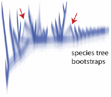
The final one is from  Figure 2 of McCormack JE, Faircloth BC, Crawford NG, Gowaty PA, Brumfield RT, Glenn TC (2012) Ultraconserved elements are novel phylogenomic markers that resolve placental mammal phylogeny when combined with species-tree analysis. Genome Research 22: 746-754.

This analysis involves bootstraps rather than Bayesian samples, showing that the same principle applies.

Evolutionary history of placental mammals resolved from conflicting
gene histories. Widespread consensus among 1000 species-tree bootstrap
replicates of the same 183-locus data set. STEAC trees are depicted because
the branch lengths allow for better visualization of branching patterns, but
STAR results supported the same topology. Cones emanating from terminal
tips of species trees (red arrows) indicate disagreement among bootstrap
replicates.

It would be nice to illustrate this further by direct comparison with a splits graph of the same dataset that I used in the previous blog post. Unfortunately, the computer program available (DensiTree) has the same practical limitation as the SplitsTree program (as mentioned in the previous post) — it does not read the MrBayes ".trprobs" file because it ignores the tree weights. This means that one has to enter the entire treefile (with thousands of trees), and I have not yet done that. Moreover, the program relies very much on having branch lengths for each tree — the output is really quite odd without them, with the taxa appearing in a series of steps rather than connected by straight branches. My previous analysis did not use branch lengths, as they are not needed for the consensus network, in which edge lengths represent support rather than character evolution.