Fossils and Networks 3 – (deleting and) adding one tip

In the last Fossils and Networks post, we explored the use of SuperNetworks to identify both safe and problematic branching patterns by removing one OTU and re-evaluating the analysis. Here, we'll take the opposite approach, and see what we can learn from adding one OTU to our analysis.

Breaking and supporting wrong branches

We start again with the artificial Felsenstein Zone matrix that results in a wrong AB clade. Here's the original true tree used to generate the matrix.

Because of convergent/parallel evolution in the modern taxa (genera O, A and B) and primitive characters of their fossil sisters, any phylogenetic inference method will find the wrong, tree with a A + B | rest split.

In the Felsenstein Zone, parsimony will always get the wrong tree due to long-branch attraction (LBA), while Maximum likelihood has a 50:50 chance to escape LBA. To break down the LBA between A and B, we need a fossil that is, from an evolutionary point of view, intermediate between D and B.

If we add a fossil E that features 1 out of 3 derived traits found in the BD lineage (including the only synapomorphy of BD), we end up with two alternative parsimony trees: one with a wrong topology and the other the correct topology, as shown here.

By adding a fossil F featuring 2 out of 3 derived traits, we increase the number of most-parsimonious trees (MPTs) to three alternatives, all of which fall prey to A-B+F LBA, as shown next.

Convergent evolution is a problem for tree inference but selection bias and homoiologies are worse, involving accumulation of the same advanced trait within some but not all members of a lineage (Has homoiology been neglected in phylogenetics?). This is worse because the characters will enforce attraction between long-branching, highly evolved (more modern) taxa. A and B are siblings, but by enforcing an ABF clade, we will inevitably misinterpret the most primitive members of the ingroup, C and D. Hence, we may draw wrong conclusions about evolution in the A–F lineage.

Because E is virtually half-way evolved between D and F, and F is the next step towards B, the all-inclusive tree gets it right. We infer a single optimal tree, shown here.

PS: Also, in this case we could use any other optimality criterion (Maximum Likelihood, Least-squares, Minimum Evolution) and we would end up with the same tree.

Missing the important bits

That last observation is encouraging: the more fossils we include in our matrix and the better they reflect the evolutionary trends within a group (here from a D-like ancestor via E to F and B), the greater the chance of ending up with the true tree. There's only one drawback: in real-world data sets, we may miss exactly those traits in the fossil sample that are needed in order to infer (or stabilize) the true tree.

(Paleo-)Parsimonists have frequently argued that missing data are unproblematic, which is true in one sense, as shown in the above example. The commonly used strict consensus tree has no wrong branches, because it only has one, which is the trivial ingroup-outgroup split. The much less commonly used Adams consensus tree has one more branch, which is wrong: the ABF clade.

As always in such cases, the strict Consensus network visualizes the MPT sample best (again exemplifying why we should stop using cladograms).

The price for not having false positives is that we cannot infer a most-parsimonious tree or a few alternative trees any more, but could easily end up with scores of them. Here, we have 41 MPTs for a 8-taxon dataset that include fairly wrong trees*, although some of them are closer to the true tree (green and olive edges in the strict Consensus network above). For large matrices, or matrices lacking tree-like signals, the number of MPTs can easily reach tens or hundreds of thousands. Lacking critical traits in E (14 out of 46 characters missing) and F (7 missing), we may escape LBA at the cost of decisiveness. If we do have those traits only in F but not E, we will enforce LBA between A and B.

Plus-1-trees (and SuperNetworks)

Before adding a taxon as an additional leaf to our tree, we may be interested in what that taxon does to our tree: can it trigger a topological change or does it fall in line? We will again take the dinosaur-to-bird-matrix of Hartman et al. (2019, PeerJ 7: e7247) as a real-world example. This includes everything from well-covered highly derived and most primitive taxa, to those that lack discriminatory signal in general (ie. are unresolved), plus the one or two rogue taxa, with ambiguous phylogenetic affinities creating topological conflict. (Note: the commonly reported strict consensus trees cannot distinguish between those two alternatives.)

The best-covered 15 taxa provide us with a single optimal tree that is in agreement with current opinion (shown below). However, this struggles to resolve the clade of modern birds because the extinct Lithornis is being attracted by Anas, the duck. When we remove Dromiceiomimus (as shown in Fossil and Networks 2), we end up with a putatively wrong Dromaeosauridae grade, because of LBA between the most distinct Dromaesauridae, Velociraptor and Bambiraptor, and the distantly related (to flying dinosaurs) Allosaurus, Tyrannosaurus and the IGM 10042 skeleton.

Two of the Minus-1 trees generated for the last post of this series.

For our experiment, we will take this (partly) wrong tree, and add every other taxon included in the Hartman et al. (2019) matrix as 15th tip. We can then perform a branch-and-bound search to infer these 14-Plus-1 tree(s). When we browse through the inferred MPTs, we can see that many taxa fall in line with the wrong topology, including a few that, in addition, increase uncertainty for branches correctly resolved in the minus-Dromiceiomimus tree.

Out of the 485 candidate trees, only 10** have a set of characters that can compensate for the missing Dromiceiomimus, leading to Plus-1 trees that show a Dromaesauridae clade, as shown here.

Two of the ten Plus-1 trees, where the added tip saves the inference from LBA. Numbers give the amount of defined characters (scored traits). Both Halszkaraptor and Zhenyuanlong are classified as Dromaeosauridae, however only the better covered taxon is placed as sister to the Dromaeosauridae included in the original 14-taxon tree.

The presence of the deep-branching Compsognathus (Tyrannoraptora: ... :Neocoelurosauria: †Compsognathidae) triggers an Archaeopteryx-Dromaesauridae clade.

In the case of relative deep-branching Garudimus (... :Neocoelurosauria: Maniraptoriformes: †Ornithomimosauria: †Deinocheiridae) and Epidexipteryx (... : Maniraptoriformes: ... : : ... : Paraves: †Scansoriopterygidae) one or two of the two or three MPTs show the wrong grade except the last the clade.

Note: the relative low number of scored traits for Epidexipteryx can avoid LBA leading to a Dromaeosauridae grade but misplace the taxon within the Plus-1 MPTs: its family, the Scansoriopterygidae, are considered to represent the sister lineage (Wikipedia, referring to Godefroit et al. 2013 Nature 498: 359–362) of the Eumaniraptora which include the Dromaeosauridae as first-diverging branch.

We can also summarize the outcome, a collection of 640 Plus-1 MPTs, in form of a z-closure SuperNetwork, as we did for the Minus-1 trees in the previous Fossils and Networks post (shown next).

This SuperNetwork is quite boxy, and may be only semi-comprehensive (I used only 20 runs, which took half a day). Matching 485 tips into a 14-taxon backbone tree is not the kind of tree sample that the SuperNetwork has originally been designed for!

Only four edges, fat and blue, are without alternatives. In all other cases, the added tip triggered the creation of several alternatives: the highest dimension for the boxes is five, but most have four or less dimensions. Regarding our problem of saving the Dromaeosauridae clade, we can see that the topological change depends on very few characters, with Microraptor being very close to the divergence but a bit more bird-like (in a very broad sense), while the other two are much more derived.

Close-up on the Dromaeosauridae part of the network, with all tips labeled. Pie charts give the percentage of scored traits/missing data. * – Tips that saved the inference from LBA (see above).

Note the length of some of the colored edges, especially the light green which represent edges reflecting a Dromaeosauridae clade. Other Dromaeosauridae taxa increase not only the diversity but also may create substantial topological ambiguity (bluish and greenish edge bundles; same color = same split) and branching bias.

Take-home message

Creating morphological supermatrixes makes a lot of sense, because it ensures normalization and facilitates universal comparability, which is crucial also for paleobiology. However, even more than molecular phylogenies, paleophylogenies are affected by character and taxon sampling. This is nothing new, and much debate has dealt with which parsimony strict consensus cladogram is the better one.

I suggest taking a new route. Instead of using morphological supermatrixes to infer trees – for this matrix, Hartman et al. found millions of equally optimal parsimony trees further filtered by post-analysis, initial tree topology informed character weighting (as implemented in TNT) – we should use it to generate subsets and engage in exploratory data analysis. This will pinpoint strengths and weaknesses of the data and its individual taxa. Rather than producing evolutionary meaningless soft polytomies, one should study the reasons for any topological ambiguity. After all, one simple reason for unstable branching patterns may be that all so-far inferred trees are biased, only differently.

The SuperNetwork can assist us in putting together taxon sets that could allow not only a simple tree inference but also topology testing.

• If we want to test the stability of, e.g., the Dromaeosauridae clade against taxon sampling, it will be of little use to include the most primitive (anything outside Maniraptora) and much more advanced taxa (Avialae including modern birds) of the 501-taxon matrix. On one had, the most primitive taxa will only increase the computational load, because our inferred tree not only optimizes branches we are interested in, but also irrelevant ones, using taxa that largely lack discriminative signal for the branches of interest or at all. On the other hand, the most derived taxa may bias the tree inference by providing strong terminal signals outcompeting potentially conflicting weak basal signals.
• If we want to test the stability of the backbone phylogeny against adding taxa and entire lineages, we may prefer short-branched over long-branched taxa, in order to avoid (local) LBA (especially when we want to stick to parsimony). The terminal edges in the SuperNetwork indicate the minimum number of unique changes for each tip added to the 14-taxon tree. As seen also in our hypothetical example: E and F only break down the wrong AB clade because both are either identical (or very similar) to the last common ancestor of E+F+B and F+B, respectively.

In a future post, I'll come back to the issue of identifying taxa that are game changers, using a simple and quick tree-based approach: the so-called "evolutionary placement algorithm", first implemented in RAxML.

PS.
For any of you who really don't like networks, but still find no comfort in comb-like strict consensus cladograms either: just tick the SuperTree option when inferring the SuperNetwork. But only if your input trees converge to a shared topology. Otherwise the result may look like this:

A SuperTree based on the 640 Plus-1 MPTs.

---

* Somebody familiar with Consensus networks and morphological data partitions providing complex signal, can extract a phylogenetic hypothesis from this boxy network for the included taxa. In general, the distance along the network edges represents a phylogenetic distance, and thus gives a direct measure of how derived a taxon is.

For example, C, D are closer to the ougroup and placed close to the centre of the graph, which is exactly where a primitive ingroup taxon, with an ancestral morphology, would be placed. F is most likely a sister of B. The olive EF | rest split supports a potential common origin of E, F, and B (long green edge bundle). Hence, A can only represent a distant, strongly evolved sister lineage (both the alternative AB and ABF clade have less character support). Also, since the graph depicts E as least derived of the four (irrespective of the topological alternatives), its affinity to F and B has more value than the affinity between A and B, both being long-branched, and hence susceptible to LBA. D fits into the picture, the olive DE edge either: (1) represents a common origin, which would make D an early member of the red lineage; or (2) has similarity due to shared primitive traits within the ingroup, which would make D an early member of an ABEF lineage. C, in contrast to D, has no clear affinities with any other ingroup member, and so can only be interpreted as an early, very primitive form with uncertain phylogenetic relationships. The (true tree) mutual monophyly of the red and blue ingroup lineages has very little character support in the matrix, and hence cannot possibly be resolved.

** Systematically they cover a range of maniraptoran ('hand hunters') families 'below' the Avialae ('flying' dinosaurs) including, in addition to two Dromaeosauridae (Halszkaraptor, Zhenyuanlong, trees shown above), members of †Alvarezsauroidea (Haplocheirus), †Caudipteridae (Caudipteryx), †Sinovenatorinae (Sinovenator), †Therizinosauroidea or related (Beipiaosaurus, Jianchangosaurus) and †Troodontidae (Gobivenator, Sinornithoides). Caihong is a member of the †Anchiornithidae, which Wikipedia flags as "Avialae ?". These OTUs show data coverage far above the median (74% missing), with 278 (Caihong) to 558 (Caudipteryx) defined characters (out of a total of 700).

Fossils and networks 2 – deleting (and adding) one tip

A general assumption in phylogenetics is: the more the better. The more data my matrix includes, the better will be my tree. The more taxa I include, the better will be my phylogenetic analysis. But is this true when we include (or rely on) fossils? After all, there is an old saying: less is more; and in this post I will show you that it is often true here, too.

Perfect data – how to recognize unproblematic topologies

In the first post of this series (Farris and Felsenstein), I introduced two matrices, a Farris Zone matrix and a Felsenstein Zone matrix, with the same set of tip taxa: three extant genera and three early fossils, one for each generic lineage.

The Farris Zone matrix provides a perfect signal. No matter which inference criterion one uses, one always gets the true tree. In such a case, the taxon sampling should be irrelevant; and it is. Any 5-taxon sub-tree correctly shows only splits found in the 6-taxon true tree — shown below are the actual most parsimonious trees (MPT) of each inference using the branch-and-bound algorithm.

Six most-parsimonious trees showing the topology of the true tree; trees are midpoint-rooted and have the same scale.
Note: NJ/LS and ML would give the same result for this experiment.

Consequently, for the perfect case, the SuperNetwork of the six 5-taxon trees is the 6-taxon true tree.

Z-closure SuperNetwork (Huson et al. 2004) of the 5-taxon MPTs generated with SplitsTree (walkthrough at the end of the post) depicting the true tree.

Therefore, the simplest test to check for potential topological issues in any set of data is to sub-sample the taxa by sequentially pruning a single taxon, infer the resulting group of trees (which I will call minus-one trees), and then summarize this tree sample in the form of a SuperNetwork. If the data have no signal issues – and the inferred all-inclusive tree is unbiased – all minus-one trees will be congruent with the all-inclusive inferred tree. The resulting SuperNetwork will then be a tree matching the inferred all-inclusive tree.

On the other hand, if removing a single taxon has a significant effect on the inferred tree, then this either means you need this taxon to get the right tree or that this taxon is causing bias. We cannot assume that trees with many taxa are better than trees with fewer taxa. Only if a topology is independent of taxon sampling can we be sure that we are looking at a true tree (or one inevitable with the data at hand).

Taxon-sampling matters? Then the all-inclusive tree may be biased

Real data matrices are far from perfect. Paleophylogenetic matrices, for instance, not only include a lot of missing data limiting the decision capacity of any phylogenetic inference, but, being restricted to morphological traits, usually high levels of homoplasy — that is, similarity in conflict or only partial agreement with the phylogeny (here are some related posts: Has homoiology been neglected in phylogeny? Should we bother about character dependency? Please stop using cladograms! The curious case[s] of tree-like matrices with no synapomorphies and More non-treelike data forced into trees: a glimpse into the dinosaurs). While some OTUs are primitive in their character suites, others are highly derived. We often, without realizing it, are infering within or close to the Felsenstein Zone.

If we repeat the same minus-one experiment, but now use the Felsenstein Zone matrix, instead, we end up with something quite different. We get three most-parsimonious tree (MPT) solutions when eliminating the outgroup genus O or its fossil Z; and eliminating the genera A and B and their fossils C and D, respectively, each leads to a single MPT. This yields a total of 10 MPTs.

First row rooted with Z, all other trees mid-point rooted. All trees have the same scale.

By pruning the long-branching genera A or B, even parsimony analysis gets the correct tree because we have eliminated the source of the long-branch attraction. Adding fossils to break down long branches can be effective (classic paper: Wiens 2005), but dropping long-branching tip taxa works just as well. Changing between a close outgroup (fossil Z) and a distant outgroup (fossil O) has little benefit here.

In this case, the resulting SuperNetwork of our 10 MPTs is not a tree but a network including alternative clades, wrong ones (orange), ie. not monophyletic, and correct ones (green) — ie. branches (internodes, bipartitions) reflecting the monophyletic lineages of the true tree.

Comprehensive Z-closure SuperNetwork of the 10 minus-one MPT inferred based on the Felsenstein Zone matrix. The network includes all split patterns found in the MPT sample.

A real world example

To give an example of how sequentially dropping one taxon works with real-world data, we'll use the exhaustive 700 character matrix for bird-related dinosaurs provided by Hartman et al. (2019).

With its total of 501 taxa (OTUs), the apparent rationale behind the matrix is that, by including as many taxa as possible, one gets the best-possible (parsimony) trees, irrespective of the signal quality provided by individual OTUs. However, the full matrix cannot be forced into a single-optimal parsimony tree, due to missing data (72% of the matrix' cells are undefined or ambiguous, ie. 255969 cells) and a scarcity of synapomorphies (in a Hennigian sense) — this is discussed in Hartman et al.; see also the related Q&A.

Here, in light of the computational effort and to avoid heuristics when searching the MPTs, we'll use a pruned sub-matrix. For our first experiment, we take 15 out of the 19 best-covered OTUs. Thus, OTU pairs / triplets that are much more similar to each other than to any other OTU, are reduced to the best-covered representative.

The 19-taxon matrix that I used in a previous post (Large morphomatrices – trivial signal) had only one most-parsimonious tree solution, showing only clades in agreement with current opinion, which assumes a largely staircase-like evolution from dinosaurs to modern birds (Tree of Life). In contrast to the full matrix, the 19-taxon matrix provided high support for most clades (method-independent), reflecting the number of scored traits. The extant taxa, representatives of modern birds (duck, turkey and ostrich, all edible), have many derived cgaracters, with the extinct bird genus Lithornis being placed in-between ostrich and duck + turkey.

The optimal topologies for the 19 best-covered taxon matrix. Green, the single most-parsimonious tree. Clade names copied from Wikipedia/Tree of Life.

The ML and NJ/LS (except for one branch) trees were topologically identical; each branch is supported by about 100 inferred changes. The signal from the matrix should be straightforward.

The tree-size weighted mean (default in SplitsTree) SuperNetwork, summarizing the result of an exhaustive branch-and-bound search using the 15-dropped-1-taxon matrices (each one resulting in a single optimal MPT) has a tree-like structure.

Allosaurus-rooted SuperNetwork of the 15 minus-one MPTs. Green – clades also found in the all-inclusive tree representing monophyla; orange – conflicting clades, blue – the all-inclusive tree doesn't resolve the assumed monophyly of modern birds, but places Lithornis as sister to Neognathae.

Conflicting clades are found in only two of the 15 inferred MPTs, being represented by short branches (their length in the other 14 trees is counted as zero).

Nonetheless, these conflicts received considerable character support. The frequency of a split in the minus-1 tree sample is irrelevant (see the A-B LBA problem discussed above — any tree including A and B showed the wrong clade). When summarizing our tree sample (especially when using MPTs), we should hence opt for a SuperNetwork, in which the edge lengths give the minimum branch lengths found in the MPT collection, ie. the edge length reflects the minimum length of the branch in all trees showing that branch.

Same SuperNetwork as above, but using the "Min" option instead of the default setting for computing edge lengths.

Without Dromiceiomimus – representing an earlier diverged lineage and step in bird evolution – the Dromaeosauridae clade, which is probably monophyletic (Wikipedia), flips and dissolves into a grade. By removing the intermediate step, we seem to create some ingroup-outgroup (long-branch) attraction.

Anas, the duck, forms the morphological link to Lithornis – with a mean morphological pairwise Hamming distance (MD) of 0.23, Anas is the most-similar OTU; and, hence, the MPT places Lithornis as sister to Anas + Meleagris (turkey; MD = 0.17). By eliminating Anas, the remaining contemporary birds form a clade — the modern birds (Neornithes) are assumed to be monophyletic but do not form a clade in the all-inclusive MPT (Struthio, the ostrich, is morphologically more distant from duck, turkey and Lithornis).

Conclusion

Even the most comprehensive, least gappy of paleophylogenetic matrices have substantial signal issues. If a tree inference is dependent on which OTUs are sampled, we cannot assume that we will automatically get better trees simply by including everything we have. Some OTUs (in our experiment: Dromiceiomimus) will stabilize correct aspects of a tree, while others will manifest bias or error (here: Anas). It's unlikely that a wrong, ie. not monophyletic, clade created by the attraction of two well-sampled taxa can be broken down by adding numerous taxa showing only a fraction of defined characters. SuperNetworks of minus-one trees can point you to the critical OTUs and unstable branching patterns of your (backbone) phylogeny.

PS. Personally, I would analyze a matrix with these properties, and a taxon sample spanning more than 150 myrs of evolution (from Allosaurus to modern birds), using ML not MP. I used MP in this post only because paleontologists are still very fond of it (not a few still discard anything else as unfit for their data). ML is less prone to long-branch attraction, results in a single tree (easier to compare when using larger taxon samples), and is speedy these days, allowing for more in-depth experiments towards the end of the exploratory data analysis. Both IQ-Tree (homepage; includes links to online servers) and RAxML-NG (open access paper providing essential links / github; implemented on various online servers) can quickly infer ML trees and establish branch support (including but not restricted to nonparametric bootstrapping) using binary and multistate data.

---

Walk-through for computing Z-closure SuperNetworks (Huson et al. 2004) in SplitsTree (v. 4, since v. 5 is still not fully functional):

1. Make sure the tree sample for reading is in Newick format, including branch-length information. The trees can be in a single file or multiple files.
2. Start SplitsTree.
3. To read in the tree sample:
   • File > Open, if your trees are in one file;
   • File > Tools > Load multiple trees, if your files (eg. minus-1 MPTs) are in different files.
4. Go to Networks > SuperNetwork. Choose "Min" for "Edge Weight" in the pop-up analysis window for the first graph. You can also try out "Mean"/"Sum" (short, rare alternatives will be less prominent), "AverageRelative" (trade-off) or "None" (branch-lengths in the minus-one tree sample are ignored). When using simple tree samples (little topological variation, matrix with fairly stringent signals), a single run (default) suffices. Increasing the number (eg. to 100) ensures no branching pattern in the minus-one tree sample gets lost. For instance, for the Felsenstein Zone matrix, a single run will give you a SuperNetwork capturing the major conflicting aspects, while 100 runs will lead to a higher dimensional graph that includes the correct BD and AC clades as alternatives. If you like to view the overall best-fitting tree instead of a network, tick "SuperTree".

---

Cited papers

Hartman​ S, Mortimer M, Wahl WR, Lomax DR, Lippincott J, Lovelace DM (2019) A new paravian dinosaur from the Late Jurassic of North America supports a late acquisition of avian flight. PeerJ 7: e7247.

Huson DH, Dezulian T, Kloepper T, Steel MA (2004) Phylogenetic super-networks from partial trees. IEEE/ACM Transactions on Computational Biology and Bioinformatics 1: 151–158.


Wiens JJ (2005) Can incomplete taxa rescue phylogenetic analyses from long-branch attraction? Systematic Biology 54: 731–742.

Supernetworks and gene tree incongruence

One of the most interesting side effects of using Big Data in phylogenetics has been the realization that individual gene trees may be wrong as an estimation of the genome phylogeny. In the past, the easy "solution" was just to add more and more gene data until any topological ambiguity disappears, leaving us with a fully resolved, all-inclusive, tree.

However, even with increasing amounts of data, some relationships remain ambiguous. Adding data sometimes reveals primary conflict in the data, eg. because of a reticulate phylogenetic history. With modern-day software, we can quickly infer trees and compare them. Less straightforward is the interpretation of the observed conflict and what to do with it.

In our The Emperor has no clothes blog mini-series [Pt 1 – the mighty matK, Pt 2 – a thicket of trees, Pt 3 – conflict or not], I discussed gene incongruence in the complete angiosperm plastome data, which some people have interpreted as evidence for inter-plastome reticulation (recombination), as well as discussing the role that a single gene may play when inferring a trees based on a concatenated, multi-gene data set.

A new analysis

In this new post, I will show what a supernetwork can tell us about gene conflict using the data from a recent (open access and open data) paper investigating deep relationships in (land) plants.

Sousa F, Civáň P, Brazão J, Foster PG, Cox CJ. 2020. The mitochondrial phylogeny of land plants shows support for Setaphyta under composition-heterogeneous substitution models. PeerJ 8:e8995.

This is what the authors state:

Majority-rule consensus trees resulting from the best-fitting Bayesian MCMC analyses of individual genes had low resolution in general, but liverworts were supported (>95% posterior probability (PP)) as the earliest-branching lineage in two genes (nad 3 and nad 5), whereas the mosses were supported as the earliest-branching lineage in one gene (ccm C). All other resolutions of the bryophyte lineages relative to the tracheophyte clade were not statistically supported, and the Setaphyta clade was not resolved in any gene tree.

The authors objective was to filter the data, leaving those genes and information that can provide a better tree — ie. a less ambiguous one, resolving the deep relationships in land plants. Filtering the additive weak signals in each gene, and countering the problem of codon bias, leads to the fully resolved, unambiguously supported concatenated tree shown below.

Sousa et al.'s fig. 2, a fully resolved (all branches have PP = 1) Bayesian tree inferred from the concatenated 36 gene amino acid data. The novelty is the unambiguous support and recognition of a Septaphyta clade composed of liverworts (turquois) and mosses (brown).

The zenodo link provides full access to the data used. It includes:

• the single-gene nucleotide and translated amino acid matrices,
• the single-gene Bayesian majority rule consensus trees (MRC)
• a concatenated 36-gene nucleotide and amino acid matrix, plus one cleaned for substitution bias ("codon degenerate"), and the resulting ML trees.

For this post, my objective is to visualize how the genes' information differs using a somewhat under-used (and under-appreciated) method: the supernetwork.

Why use a Supernetwork

Typically, we might just display the Consensus network of the single-gene trees (eg. summarizing branch-lengths or using averaged branch-lengths), and then compare it to the "preferred" concatenated tree (above). But, the data at hand includes missing gene partitions: some gene trees have fewer leaves. Consensus networks need tree samples that all have the same set of tips, while Supernetworks, on the other hand, can handle trees with different tip sets.

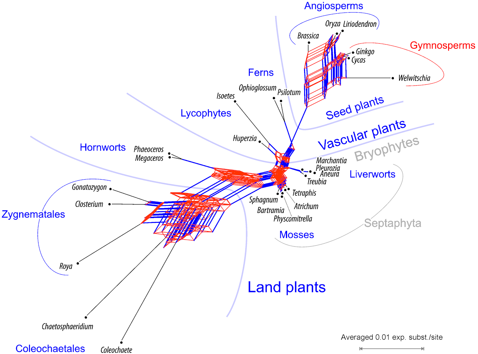
Here is the Supernetwork for our data, using the z-closure algorithm and tree-size averages for edge lengths (Huson et al. 2004, IEEE/ACM Trans. Comput. Biol. Bioinform. 1: 151–158).

Supernetwork of the 36 mitochondrial gene trees. Edge bundles corresponding to branches in Sousa et al.'s fully resolved tree in blue, conflicting edge bundles in red. Gray, systematic groups not represented by according branches (taxon bipartitions) in any gene tree.

This Supernetwork is not based on the MRC provided, but gene-based ML trees. MRC trees are not strictly phylogenetic trees (Losing information in phylogenetic consensus; Why should we present a Bayesian phylogenetic analyses using networks): they can include, as in this case, polytomies originating from collapsing branches below a certain PP threshold. To distill and visualize the primary (raw) signal, I also did not partition the codons; treating the often saturated (in the case of mt DNA) third codon position as distinct data partition, would be obligatory in case we wanted to have the best-possible phylogenies.

Although the network is quite boxy (not tree-like), it does contain nearly all of the edges (branches; in blue) that make up Sousa et al.'s fully resolved, concatenated amino acid tree, with the exception of the Septaphyta edge (as noted by Sousa et al.) Although we used the suboptimal nucleotide matrices and none of our gene trees was fully congruent with the concatenated amino acid tree, they all included aspects of it (despite not filtering or correcting for codon bias).

When talking about gene incongruence, use a Supernetwork

Supernetworks (see also Whitfield et al. 2008, Syst. Biol. 57: 939–947) are much under-used graphs, ideal to visualize statements such as the one by Sousa et al. quoted above. They not only show the full extent of the gene tree incongruence but also to what degree it relates to short or long branches in the gene trees — this is something that, eg., cloudograms, fail to do. While a cloudogram is a summary of cladograms (sister relationships), a Supernetwork is a summary of phylograms, phylogenetic trees informing us about the amount of change. Keeping an eye on branch lengths helps a lot when interpreting branch support and discussing tree topologies, especially trees based on concatenated gene data (filtered or not).

The network of woodpeckers, etc

The world continues on its merry way, searching for fragments of the Tree of Life. That is, research papers continue to be published that give no credence to the possibility of reticulate evolutionary history, especially in zoology.

A recent case in point is this one:

Matthew J. Dufort (2016) An augmented supermatrix phylogeny of the avian family Picidae reveals uncertainty deep in the family tree. Molecular Phylogenetics and Evolution 94: 313–326.

The author constructed a supermatrix for 26 loci for 78 taxa of the bird family containing woodpeckers, piculets, and wrynecks. The author used an array of phylogenetic techniques, including the construction of maximum-likelihood "gene" trees, several different maximum-likelihood species trees, plus time trees. All of these methods pre-suppose that the evolutionary history of the species was strictly tree-like.

We can use an exploratory data analysis to evaluate how probable is this fundamental assumption. I constructed a SuperNetwork based on the 26 gene trees produced by the author, using the SplitsTree program, as shown here. The network is basically tree-like, with one major exception.

I have labeled only one taxon, which seems to be the culprit for the major non-tree-likeness. This species appears in 10 of the gene trees, being part of the Leiopicus group (as expected) in 7 of the rooted trees. It is unexpectedly related to the Picus group in two of the other rooted trees, and is close to Dryocopus in the remaining tree.

This network EDA does not, of course, imply the existence of reticulate evolution. It does, however, highlight a pattern of incongruence that requires explanation, if the history of these birds is to fully elucidated. Reticulate evolution remains one of the possible explanations, pending further investigation.

For an example of a network view of bird evolution, see:

Antonio Hernandez-Lopeza, Didier Raoult, Pierre Pontarotti (2013) Birds perching on bushes: networks to visualize conflicting phylogenetic signals during early avian radiation. Comptes Rendus Palevol 12: 333-337.

Lager beer and phylogenetic networks

Beer and wine making have been known since ancient times, but both were usually a hit-or-miss affair. However, beer brewing gradually changed during the Middle Ages in Europe to produce a consistent ale-type beer. The process is carried out by the yeast Saccharomyces cerevisiae, which is also involved in producing wine and leavened bread.

Lager beer, on the other hand, was first brewed in the 15th century in Bavaria (now part of Germany), and it has since become the most popular type of beer worldwide. Lager is bottom fermented (versus top-fermented for ale), and the fermentation is carried out at a lower temperature (< 10 °C versus 15-25 °C). It produces a "smooth, crisp, fruity, and clean" beer as opposed to the "robust, hearty and fruity" ale beer.

Lager beers are made using a yeast known as Saccharomyces pastorianus (also known as Saccharomyces carlsbergensis). This is a domesticated species that depends on humans for its propagation, and it is an allotetraploid hybrid. For a long time, we have known that half of the genome came from the ale yeast Saccharomyces cerevisiae, but the other half came from an unidentified species. In 2011, Libkind et al. (Microbe domestication and the identification of the wild genetic stock of lager-brewing yeast. Proceedings of the National Academy of Sciences of the USA 108: 14539-14544) identified the missing parent yeast as the previously unknown species Saccharomyces eubayanus, which grows on Nothofagus (Southern Beech) trees in Patagonia (in Argentina).

Lager was developed when the Bavarians started to brew and store their beer in caves or cellars, which kept it at a constant cool temperature. This required a yeast that could tolerate the colder temperatures, and it is apparently this component that Saccharomyces eubayanus contributes to the Saccharomyces pastorianus hybrid. Precisely how it got from Patagonia, at the southern tip of South America, to south-eastern Germany is not clear, but perhaps some were carried on the feet of fruit-flies.

Since we are dealing with an allotetraploid hybrid, and thus reticulate evolution, a phylogenetic network would be the appropriate means to illustrate its origins. This has recently been provided by Peris et al. (2014. Population structure and reticulate evolution of Saccharomyces eubayanus and its lager-brewing hybrids. Molecular Ecology 23: 2031-2045). They report that:

genetically diverse strains of S. eubayanus are readily isolated from Patagonia, demonstrating that the species is well established there. Analyses of multilocus sequence data strongly suggest that there are two diverse and highly differentiated Patagonian populations. The low nucleotide diversity found in the S. eubayanus moiety of hybrid European brewing strains suggests that their alleles were drawn from a small subpopulation that is closely related to one of the Patagonian populations ... These findings show how genetically diverse eukaryotic microbes can produce rare but economically important hybrids with low genetic diversity when they migrate from their natural ecological context.

The authors actually present two networks, the first of which is shown here. It is an unrooted supernetwork derived from the the maximum-likelihood trees of each of eight nuclear genes. It shows the network of samples from three named Saccharomyces species, along with expanded views of the two Patagonian populations. Isolates W34/70 and BCS1503 are from the lager yeast, Saccharomyces pastorianus, which in the network are related to the Patagonia B population. The three Saccharomyces bayanus samples (beer contaminants) are hybrids between Saccharomyces eubayanus and Saccharomyces uvarum.

Is this the first network from conflicting datasets?

There are no new problems in science, only old ones that obtrude themselves on you in new ways. One biological example of this truism is the discovery by molecular biologists that different genetic datasets produce different phylogenetic trees. This has been known at the phenotypic level for centuries, so that systematists have used reticulating structures such as maps, networks, webs etc to try to display the many different ways in which biological organisms appear to be related to each other, with different relationships shown by different parts of the phenotype.

This multi-faceted nature of relationships became problematic after 1859, when biologists more-or-less settled on trees as a means of displaying genealogy, because trees show only one set of relationships. Indeed, Darwin himself (1851, 1859) noted that different organ systems suggest different relationships. However, he believed that a taxonomic classification should be based on the structure of the entire body, not just one organ system, so that all relationships are considered. He thus concluded that it is necessary to give each kind of feature a different "weight" in contributing to the overall scheme, both for working out phylogenies and for erecting classifications based on them.

Darwin did no explicit phylogenetic work of his own, and so it was St George Mivart who first had to deal with this situation empirically (as discussed this previous blog post). His early work was principally on the comparative anatomy of primates, for which he provided very detailed comparisons of the skeletons of a large number of species, notably in Mivart (1865), based on the axial skeleton (or spinal column), and Mivart (1867), based on the appendicular skeleton (or limbs).

In the 1865 paper Mivart noted that the data for the spinal column "lead to an arrangement of groups and an interpretation of affinities somewhat differing from, yet in part agreeing with, the classification founded on cranial and dental characters". Moreover, the 1865 and 1867 studies did not produce the same phylogenetic tree. Mivart explicitly noted in a letter to Darwin (1870): "The diagram in the Pro. Z. Soc. [1865] expresses what I believe to be the degree of resemblance as regards the spinal column only. The diagram in the Phil. Trans. [1867] expresses what I believe to be the degree of resemblance as regards the appendicular skeleton only" (Darwin Correspondence Project, letter 7170).

In the modern world, one way to deal with this sort of data conflict is to use a phylogenetic network rather than a phylogenetic tree. That is, we do not need to produce a consensus classification based on weighting different datasets (as suggested by Darwin), and we do not need to produce a series of conflicting trees (as done by Mivart). We do not even need to produce a consensus tree, which would be a combination of these two approaches. We can, instead, display the conflict among the different data sources in a single diagram, as a network.

Click to enlarge.

Here, I have produced a network based on Mivart's 1865 and 1867 trees. There are 24 taxa of Primates, although the Gorilla was not in the 1865 dataset, and Inuus, Cynocephalus, Chrysothrix were not in the 1867 dataset. From these two trees I have produced a SuperNetwork, using the SplitsTree program. This is thus a splits graph, interpreted in the usual manner, so that the reticulated parts represent conflict between the two trees and the non-reticulated parts represent agreement.

The main conflict between the two trees is in the relationship between the Nycticebinae and Cebidae, shown as the centre reticlulated area in the network. Basically, the root of Mivart's trees is between these two groups, and they swap sides of the root between 1865 and 1867! Another cause of this netted area is whether Homo is within the Simiinae (as in the 1865 tree) or sister to the Apes (as in the 1867 tree). These two sources of conflict are quite major, from the biological point of view.

The bottom netted area of the network is caused by conflicts about relationships within the Lemuroidea, which are of less consequence. The top netted area refers to whether Simia is sister to either Hylobates (in 1867) or Troglodytes (in 1865), which is a relatively minor point.

It is tempting to see Mivart's change in the position of Homo (from 1865 to 1867) as psychological rather than empirical. Mivart came to reject the idea that humans should be placed in a phylogenetic tree, and expressed this strongly in Mivart (1871). He then became a strong opponent of Darwinian evolution for a time. Nevertheless, he returned to the fold at least once, in Mivart (1881), where he presented a phylogenetic tree of much of the Mammalia, based on dentition. However, he conspicuously excluded the Primates from this tree, thus dodging the theological problem entirely.

Note: For another early example see Fritz Müller and the first phylogenetic tree.

References

Darwin, C. (1851) A Monograph of the Sub-Class Cirripedia, with figures of all the species. The Ray Society, London.

Darwin, C. (1859) On the Origin of Species by Means of Natural Selection. John Murray, London.

Mivart, St.G. (1865) Contributions towards a more complete knowledge of the axial skeleton in the primates. Proceedings of the Zoological Society of London 33: 545-592.

Mivart, St.G. (1867) On the appendicular skeleton of the primates. Philosophical Transactions of the Royal Society of London 157: 299-429.

Mivart, St.G. (1871) On the Genesis of Species. Macmillan, London.

Mivart, St.G. (1881) The Cat: An introduction to the study of backboned animals, especially mammals. John Murray, London.