
In a recent paper published in Systematic Biology, Joseph O’Reilly and Philip Donoghue (2017) shed some light on an issue concerning Bayesian analysis that has also bugged me since I first crossed paths with total evidence dating. Should we put dates on trees with topologies that may be “spurious”? Their answer is: "better not to". Based on their results, they advocate the use of majority-rule consensus trees (MRC), because maximum credibility clade (MCC) and maximum a posteriori (MAP) topologies may contain a critical number of erroneous branches.
I agree; but, being a notorious fan of non-trivial signals, in this post I will outline why one should generally use support consensus networks (SCN) to summarize the Bayesian tree sample, and then decide on those topological alternatives that are worth dating.
What O’Reilly and Donoghue found, and a simulation example
Using a series of simulated binary matrices and empirical datasets, these authors conclude that MCC trees, most commonly used by researchers doing total evidence (TE) or fossilized birth-death tip dating (FBD-TD), and MAP trees (rarely seen, but a reviewer asked the authors to include them, too) may contain too many erroneous branches (Fig. 1 provides an example). Low posterior probabilities are an alarm signal that should not be ignored. Being most conservative when it comes to accepting clades, MRC trees are hence less problematic.
 |
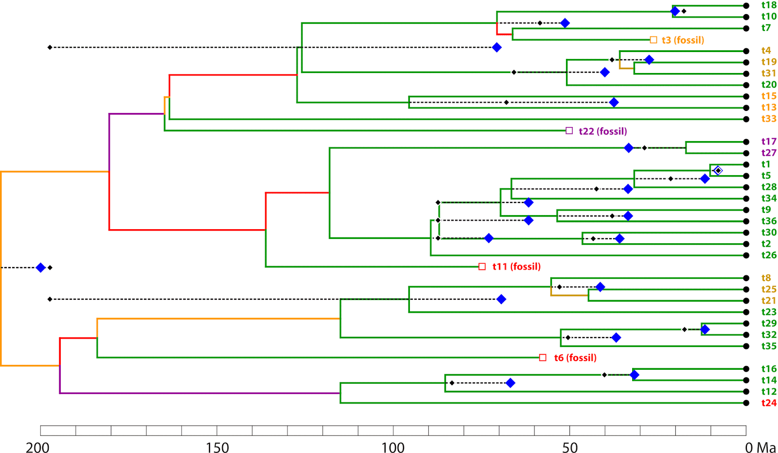
| Fig. 1 Tanglegram showing the true tree (left) in comparison to the inferred MCC tree. |
But the problem naturally goes deeper: why can we have erroneous branches, and more importantly, low posterior probabilities?
When you have worked with a lot of messy datasets (ie. data with complex signal), you may have noticed that the optimized trees are not necessarily showing the best-supported splits. This also applies to ML optimizations, and molecular datasets (see example in my recent post). Morphological data are an especially challenging problem (post1/post2/post3/…). For the example in Fig. 1, the first of 10,000 MCCs O’Reilly and Donoghue inferred based on simulated data, it seems that:
- all fossils are misplaced, some severely, but with consistently low support;
- all deeper branches, branches near to the root, are (more or less) wrong.
The prime problem: morphological data matrices provide no tree-like signals
With a matrix Delta value of 0.37, the matrix falls within the usual range seen in real-world morphological matrices, providing mainly non-treelike signals. The Neighbour-net (Fig. 2) is consequently boxy, with the central part approaching a spider-web — a very common structure when analyzing real-world morphological matrices. The Neighbour-net thus explains why the Bayesian MCC tree (and the Bayesian optimization in general) fails so miserably regarding some branches but not others.
 |
| Fig. 2 Neighbour-net based on mean morphological distances estimated from the matrix used for the Bayesian inference. Edge-bundles corresponding to branches in the true tree are highlighted in green. |
The Neighbour-net includes several prominent edge-bundles matching more terminal relationships in the true tree. In these cases, the matrix provides strong, coherent signal, as also expressed in nearly unambiguous PPs. Some taxa such as t23, t24, and t33 provide quite ambiguous signals, and they are accordingly misplaced in the MCC tree — this is the reason for very low PP in the corresponding portion of the tree.
Regarding the fossils:
- Tip-close fossil t3, an extinct sister lineage of clade {t7 + [t10+t18]} is clearly a close relative of the latter, which is something also resolved in the MCC (slightly wrong but with low support; Fig. 1) and MRC trees (where t3, t7, and t10+t18 would be part of a soft polytomy)
- t11 seems to have some weak and misleading affinity to t17+t27 (compare with Fig. 1);
- t6 is correctly placed in between clade {t12 + [t14+t16]} and clade t8–t35; and
- t22 could be interpreted as an early side lineage of the latter clade (t8–t35), too, which is not too wrong with respect to its position in the true tree (but wrong in the MCC tree; Fig. 1).
 |
| Fig. 3 The topology of the MRC (Bayesian majority-rule consensus tree) in relation to the distance-based Neighbour-net. |
Why consensus networks are without alternative
The standard MRC trees would collapse, to so-called “soft” polytomies, all of the erroneous branches in this example, plus a few correct ones (Fig. 3). This avoids the problem of misleading branches; but it comes with the cost that we cannot establish a sensible phylogenetic hypothesis and may even lose correct branches (four in the example). The 50%-MRC tree for the example in Fig. 1 would have 14 clades / terminals emerging from the soft root polytomy, which would leave us with (14-2)² = 144 topological alternatives — this is too many to consider. Consensus networks can reduce these options (Fig. 4). Plus, they inform us of whether a low support value is due to lack of discriminating signal or to conflicting signal. In the case of the simulated data, it’s naturally more the latter.
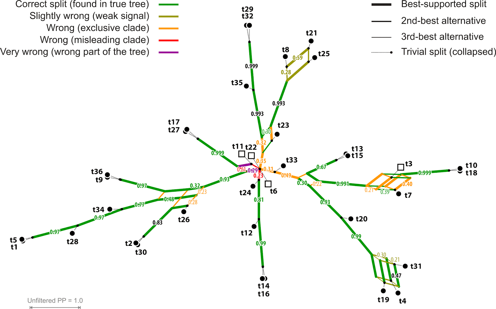 |
| Fig. 4 SCN (support consensus network) based on 10,000 Bayesian sampled topologies (BST) O'Reilly & Donoghue inferred for their simulated data set Mk100/1. Splits found in less than 20% of the BST not shown; trivial splits collapsed. This sample was the basis for selecting the MCC (Fig. 1) and computing the MRC (Fig. 3) trees. Note how the soft polytomies in the MRC can be resolved into few competing alternatives. |
Total-evidence can circumvent this problem to some degree, because the molecular data (in the optimal case) will constrain a backbone topology, which the morphological partition will have to fit into. Bayesian inference eliminates internal data conflict, as the chain optimizes towards a topology, or set of topologies, that best explain all data. This can have a streamlining effect on deep relationships, where the signal from the morpho-matrix is usually diffuse, but also towards the terminals. Here, the putative convergences conflicting with the molecular tree will be effectively down-weighted during the optimization.
Nevertheless, there are limitations. When the fossils show overall primitive or well-mixed character suites, there will be more than one possible placement. The consequence is topological ambiguity expressed in split support patterns. This is also the case for many fossils included in the dataset used in the original study introducing Bayesian TE dating (Ronquist et al. 2012), and as empirical examples in O’Reilly & Donoghue's assessment of MCC, MRC, and MAP trees.
 |
Fig. 5 SCN (support consensus network) based on the 1000 last BST of both runs performed by O'Reilly & Donoghue on the full data set of Ronquist et al. (2012).
Blue edges refer to the branches seen in Ronquist et al.'s dated MRC tree (their fig. 7); modern-day groups and potential fossil members (open squares) coloured according to Ronquist et al. (2012: fig. 3). Filled circles: modern-day taxa. Note the prefential placements for a number of fossil taxa, which formed part of large, soft polytomies in the dated MRC tree. For instance, Palaeathalia, a fossil with highly ambiguous signal, is unresolved within the Tenthredinoidea clade in the MRC trees (emerges from a pentatomy, i.e. 52 = 25 principal topological alternatives). Based on the SCN, the number can be reduced to ten alternatives, which boiled down to three principal ones: sister to Tentredinidae, Blasticotomidae or all of Tenthredinoidea except for Blasticotomidae. The latter potentially including two additional fossils that are also part of the Tenthredinoidea pentatomy.
|
This is also the reason why we relied on fossilized birth-death dating for the Osmudaceae (Grimm et al. 2015). The earliest (Jurassic) representatives of the modern Osmundaceae (= Osmundeae according Bomfleur et al. 2017) that could be included in the total-evidence matrix shared many rhizome traits with the least-derived extant lineages (genera Claytosmuna and Osmunda; PPG I 2016). The signal from the morphological partition is not tree-like (see Bomfleur et al. 2015, fig. 8) and the total-evidence MRC accordingly collapsed with only the position of a single (unambiguous) rhizome fossil (Todea tidwellii) being fully resolved (Fig. 6).
 |
| Fig. 6 Total-evidence (TE) dating (Grimm et al. 2015) using the oligogene data by Metzgar et al. (2008; resulting in a fully resolved, unambiguously supported tree) combined with a morphological partition scording for rhizome traits of modern Osmundaceae (= Osmundeae according Bomfleur et al. 2017). Four issues hinder the application of TE dating for this data set: 1. Poor backbone resolution (low, ambigous PP) preferring misleading relationships (cf. Bomfleur et al. 2015, 2017; Grimm et al. 2015). 2. The extant members of genera Claytosmunda, Osmunda, Plenasium are embedded in a large soft polytomy including fossils with the more primitive Claytosmunda-Osmunda rhizome morphologies. 3. Jurassic representatives of Osmundastrum (likely monophyletic) and Claytosmunda (paraphyletic according Bomfleur et al. 2017) form a poorly resolved "basal grade". 4. First representatives of Claytosmunda, Osmundastrum, and the Todea-Leptopteris lineage can be found in the Triassic, but cannot be included in a TE tree-inference framework (Bomfleur et al. 2017, fig. 15, section 2.2.3). |
 |
| Fig. 6 (ctd) The results of fossilized-birth death datings that used only the frond (not used for TE dating) or rhizome fossils (same set than used for TE dating). Osmundaceae foliage (sterile and fertile fronds) can be very characteristic and be traced in the fossil record, but provides only very few scorable traits. Shown chronograms modified from Grimm et al. (2015), supplement-fig. S2. Todinae: L. = Leptopteris, T. = Todea; Osmundinae: C. = Claytosmunda, O. = Osmunda, Om = Osmundastrum, P = Plenasium (cf. PPG I 2016; Bomfleur et al. 2017) |
Shall we stop using TE dating?
Naturally, dating a MRC tree with large, deep polytomies (Figs 5, 6) will not be very revealing (Fig. 7). So, even though they are much less prone to error than MCC trees, they don’t provide a practical alternative. However, by using the SCN (support consensus network) we can:
- depict the most likely (in a literal sense) topological alternatives (evolutionary scenarios);
- constrain their main aspects;
- date each of the resulting evolutionary scenarios; and
- compare the outcome.
 |
| Fig. 7 Variation in total-evidence dating estimates for the simulation example in Fig. 1 (O'Reilly & Donoghue's matrix Mk100/1). The scale has been adjusted to fit the fossils' relative ages and assuming an actual (real) root age of 200 million years (Ma). Shown is the MCC chronogram, the estimates of corresponding nodes according to the equally scaled MRC tree (black diamonds), and the target divergence ages (blue diamonds) according to the true tree (the tree used to simulate the data). The saturation of the morphological partition triggers too long terminal branches in both the MCC and MRC trees, hence, most mid-topology estimates are overestimating. MRC-derived estimates can be better than MCC estimates, but also much worse due to collapsed soft polytomies. Note that in the case of real-world data, the molecular partitions may compensate for the branching-length bias to some degree (see also Fig. 6). |
Furthermore, the SCN will point us to the ‘weak spots’ in our fossil-inclusive phylogeny, and also to the rogues — fossils with strongly ambiguous (non-treelike) signal that mess up any tree inference. For dating, we need a tree, and hence a set of taxa providing a tree-like-as-possible signal (see the reduced data set used in Ronquist et al. 2012 for the in-text figures). For all other data sets, where ambiguous signal from fossils and morphology is inevitable, the (original) fossilized birth-death dating remains the best option.
However, be careful with the new tip-dating option, because this again assumes that the position of fossils can be unambiguously optimized in the tree.
One thing is clear: (largely) ignoring the fossil record when doing molecular dating to infer organismal histories is the worst of all possibilities.
Thanks
To Joe O'Reilly for providing the Bayesian result files (BST samples, MCC and MRC trees) used in their study.
Related posts
Why we should use consensus networks to summarize Bayesian analysis:
- concept and references — We should present bayesian phylogenetic analyses using networks
- practical aspects — How to construct a consensus network from the output of a bayesian tree analysis
- example (mosasaurs) — Networks, not trees, identify "weak spots" in phylogenetic trees
Non-treelike morphological data used to infer (strict) consensus trees:
- dinosaurs — More non-treelike data forced into trees: a glimpse into the dinosaurs
- spermatophytes — Should we try to infer trees on tree-unlikely matrices?
References
Bomfleur B, Grimm GW, McLoughlin S. 2015. Osmunda pulchella sp. nov. from the Jurassic of Sweden—reconciling molecular and fossil evidence in the phylogeny of modern royal ferns (Osmundaceae). BMC Evolutionary Biology 15:126. http://dx.doi.org/10.1186/s12862-015-0400-7
Bomfleur B, Grimm GW, McLoughlin S. 2017. The fossil Osmundales (Royal Ferns)—a phylogenetic network analysis, revised taxonomy, and evolutionary classification of anatomically preserved trunks and rhizomes. PeerJ 5:e3433. https://peerj.com/articles/3433/
Grimm GW, Kapli P, Bomfleur B, McLoughlin S, Renner SS (2015) Using more than the oldest fossils: dating Osmundaceae with the fossilized birth-death process. Systematic Biology 64: 396–405.
Grímsson F, Kapli P, Hofmann C-C, Zetter R, Grimm GW (2017) Eocene Loranthaceae pollen pushes back divergence ages for major splits in the family. PeerJ 5: e3373. https://peerj.com/articles/3373/
Metzgar JS, Skog JE, Zimmer EA, Pryer KM. 2008. The paraphyly of Osmunda is confirmed by phylogenetic analyses of seven plastid loci. Systematic Botany 33:31–36.
O'Reilly JE, Donoghue PCJ (2017) The efficacy of consensus tree methods for summarising phylogenetic relationships from a posterior sample of trees estimated from morphological data. Systematic Biology https://academic.oup.com/sysbio/advance-article-abstract/doi/10.1093/sysbio/syx086/4587515
PPG I. 2016. A community-derived classification for extant lycophytes and ferns. Journal of
Systematics and Evolution 54(6):563–603 http://onlinelibrary.wiley.com/doi/10.1111/jse.12229/epdf
Ronquist F, Klopfstein S, Vilhelmsen L, Schulmeister S, Murray DL, Rasnitsyn AP (2012) A total-evidence approach to dating with fossils, applied to the early radiation of the hymenoptera. Systematic Biology 61: 973–999.
No comments:
Post a Comment