The origin of an idea: reducing networks to trees

I have written a number of times in this blog about the strong tendency for people to present reticulating evolutionary relationships as trees rather than as networks. This involves them somehow reducing complex networks to bifurcating trees.

When referring to a "family tree", the most common way to reduce a network to a tree is simply to repeat people's names as often as necessary. That is, rather than have them appear once (representing their birth) with multiple reticulating connections representing their reproductive relationships, they appear repeatedly, once for their birth and once for each relationship, so that there are no reticulations. I presented a number of online examples of this process in my posts on Reducing networks to trees and on Thoroughbred horses and reticulate pedigrees.

Recently, Jean-Baptiste Piggin has pointed out that this approach actually has a very long history, indeed, actually dating back to what seems to be the first pictorial representation of a genealogy.

In an earlier post (The first infographic was a genealogy) I described Piggin's work on what he calls the Great Stemma, a diagram from c. 400 CE (Late Antiquity) representing the genealogy of Jesus as presented in the New Testament. In a recent update, Piggin reports:

The Great Stemma contains 13 doppelganger or fetches, that is to say, simultaneous appearances of the same person in two places, e.g. Hezron [as a] child, and separately as an ancestor of Jesus. This graphic method simplifies the layout, but forced the Late Antiquity reader to mentally register these virtual "hyperlinks".

If you view his diagram of the Great Stemma (Touring the Reconstruction), you can see on an overlay a set of links connecting the multiple appearances of the following people:
Athaliah, Gershon, Hezron, Judah, Kohath, Leah, Levi, Mahalath, Merari, Perez, Rachel, Rebekah, and Timna.

This repetition simplifies what is a rather complex diagram, which actually shows a network of family relationships. There is still one reticulation in the diagram, however, because it depicts Jesus' ancestry as described in the New Testament by both Matthew (labeled Filum C in the schematic below) and Luke (labeled Filum D), and these differ regarding the descendants of David (but not his ancestors).

The diagram contains more than just a genealogy (represented by Filum A-D), as it also displays other references from the Bible (indicated in yellow). Piggin is still working on his reconstruction (there are no known copies of the original, only later hand copies), and he continues to make discoveries.

Of especial interest in the genealogies is that Piggin now reconstructs the Great Stemma as having a strictly grid-like arrangement of the people, as discussed in his blog post Secret of the oldest infographic revealed: a grid. The placements of the lineages in the Stemma, and the connections between the people, are not always obvious to modern eyes (see my post on How confusing were the first written genealogies?), since we are used to the modern version of a "family tree" — it took another millenium after the Stemma to settle on the modern version. However, the use of a regular grid-like arrangement in the Stemma seems surprisingly modern by comparison.

Unfortunately, this arrangement seems to have become corrupted in the subsequent hand-made copies, suggesting that the scribes did not always appreciate the grid's organizational importance.

Once more on artificial intelligence and machine learning

In an earlier blog post, I expressed my scepticism regarding the scientific value of non-transparent machine learning approaches, which only provide a result but no transparent explanation of how they arrive at their conclusion. I am aware that I run the risk of giving the impression of abusing this blog for my own agenda, against artificial intelligence and machine learning approaches in the historical sciences, by bringing the problem up again. However, a recent post in Nature News (Castelvecchi 2016) further substantiates my original scepticism, providing some interesting new perspectives on the scientific and the practical consequences, so I could not resist mentioning it in my post for this month.

Deep learning approaches in research on artificial intelligence and machine learning go back to the 1950s, and have now become so successful that they are starting to play an increasingly important role in our daily lives, be it that they are used to recommend to us yet another book that somebody has bought along with the book we just want to buy, or that they allow us to take a little nap while driving fancy electronic cars and saving carbon footprints for our next round-the-world trip. The same holds, of course, also for science, and in particular for biology, where neural networks have been used for tasks like homolog detection (Bengio et al. 1990) or protein classification (Leslie et al. 2004). This is true even more for linguistics, where a complete subfield, usually called natural language processing, has emerged (see Hladka and Holub 2015 for an overview), in which algorithms are trained for various tasks related to language, ranging from word segmentation in Chinese texts (Cai and Zhao 2016) to the general task of morpheme detection, which seeks to find the smallest meaningful units in human languages (King 2016).

In the post by Castelvecchi, I found two aspects that triggered my interest. Firstly, the author emphasizes that answers that can be easily and often accurately produced by machine learning approaches do not automatically provide real insights, quoting Vincenco Innocente, a physicist at CERN, saying:

As a scientist ... I am not satisfied with just distinguishing cats from dogs. A scientist wants to be able to say: "the difference is such and such." (Vincenco Innocente, quoted by Castelvecchi 2016: 22)

This expresses precisely (and much more transparently) what I tried to emphasize in the former blog post, namely, that science is primarily concerned with the questions why? and how?, and only peripherally with the question what?

The other interesting aspect is that these apparently powerful approaches can, in fact, be easily betrayed. Given that they are trained on certain data, and that it is usually not known to the trainers what aspects of the training data effectively trigger a given classification, one can in turn use algorithms to train data that will betray an application, forcing it to give false responses. Castelvecchi mentions an experiment by Mahendran and Vedaldi (2015) which illustrates how "a network might see wiggly lines and classify them as a starfish, or mistake black-and-yellow stripes for a school bus" (Castelvecchi 2016: 23).

Putting aside the obvious consequences that arise from abusing the neural networks that are used in our daily lives, this problem is surely not unknown to us as human beings. We can likewise be easily betrayed by our expectations, be it in daily life or in science. This, finally, brings us back to networks and trees, as we all know how difficult it is at times to see the forest behind the tree that our software gives us, or the tree inside the forest of incompletely sorted lineages.

References

• Bengio, Y., S. Bengio, Y. Pouliot, and P. Agin (1990): A neural network to detect homologies in proteins. In: Touretzky, D. (ed.) Advances in Neural Information Processing Systems 2. Morgan-Kaufmann, pp. 423-430.
• Cai, D. and H. Zhao (2016) Neural word segmentation learning for Chinese. In: Proceedings of the 54th Annual Meeting of the Association for Computational Linguistics, pp. 409-420.
• Castelvecchi, D. (2016): Can we open the blackbox of AI. Nature 538: 20-23.
• Hladka, B. and M. Holub (2015 A gentle introduction to machine learning for natural language processing: how to start in 16 practical steps. Lang. Linguist. Compass 9.2: 55-76.
• King, D. (2016) Evaluating sequence alignment for learning inflectional morphology. In: Proceedings of the 14th Annual SIGMORPHON Workshop on Computational Research in Phonetics, Phonology, and Morphology, pp. 49–53.
• Leslie, C., E. Eskin, A. Cohen, J. Weston, and W. Noble (2004) Mismatch string kernels for discriminative protein classification. Bioinformatics 20.4: 467-476.
• Mahendran, A. and A. Vedaldi (2015) Understanding deep image representations by inverting them. In: 2015 IEEE conference on computer vision and pattern recognition (CVPR), pp. 5188-5196.

Grape harvest dates as proxies for global warming

Phenological patterns are often highly correlated with temperatures. As noted by Chuine et al. (2004):

Biological and documentary proxy records have been widely used to reconstruct temperature variations to assess the exceptional character of recent climate fluctuations. Grape-harvest dates, which are tightly related to temperature, have been recorded locally for centuries in many European countries. These dates may therefore provide one of the longest uninterrupted series of regional temperature anomalies (highs and lows).

Harvest dates of grapes in western Europe (used for wine-making) are of especial interest because they constitute long phenological records, as a result of the fact that the harvest dates are usually officially decreed, based on the ripeness of the grapes. In other words, we have historical records for many locations over many years.

Daux et al. (2012) have compiled many of these records into a publicly accessible database archived at the World Data Center for Paleoclimatology.

This database comprises time series for 380 locations, mainly from France (93% of the data) as well as from Germany, Switzerland, Italy, Spain and Luxembourg. The series have variable lengths up to 479 years, with the oldest harvest date being for 1354 CE in Burgundy. The series are grouped into 27 regions "according to their location, to geomorphological and geological criteria, and to past and present grape varieties." These regions are shown in the map.

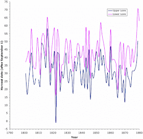
Normally, such data would simply be graphed as a time series for each region. However, as usual in this blog, we can examine these data using a phylogenetic network, to perform an exploratory data analysis. However, most of the data are actually "missing", because most of the time series have time gaps or cover only short periods. So, to create a more complete dataset I have extracted the data for the years 1800-1880, inclusive, because for this period 17 of the regions have mostly a complete series.

Two of the time series are shown in the first graph. This shows that the two time series are highly correlated, as are most of them. In this case, the correlation coefficient is 0.87.

I then used the gower distance to calculate the similarity of the different years and regions, based on the harvest dates (the gower measure is needed in order to deal with the fact that some of the data are still missing). This was followed by a neighbor-net analysis to display the between-region and the between-year similarities as two phylogenetic networks.

Only the first network is shown here. Regions that are closely connected in the network are similar to each other based on the variation in their harvest dates through time, and those that are further apart are progressively more different from each other.

Many of the patterns here are to be expected, based on the geographical proximities of the regions, but some are not. For example, Ile de France, Champagne and Vendée - Poitou Charente are all in northern France (see the map) while Bordeaux is in the south-west, and the Rhone Valley regions are in the south-east. As Le Roy Ladurie & Baulant (1980) have noted, the vineyards of northern and central France are in a different climatic zone from the wine regions of southern France (to the south of the Geneva parallel) and those of western France (west of the Chateau-du-Loire meridian).

Similarly, at the other end of the network, the Lower Loire region is not geographically located near any of the associated regions in the network. Possibly the most unexpected pattern, then, is the network separation of the Upper and Lower regions of the Loire Valley, which are the two regions whose time series are graphed above.

Clearly, the network is displaying only quite small differences between the time series. That is, the time patterns are very consistent across the regions, which does indeed make them useful for studying past temperature patterns.

References

Isabel Chuine, Pascal Yiou, Nicolas Viovy, Bernard Seguin, Valérie Daux, Emmanuel Le Roy Ladurie (2004) Grape ripening as a past climate indicator. Nature 432: 289-290.

V. Daux, I. Garcia de Cortazar-Atauri, P. Yiou, I. Chuine, E. Garnier, E. Le Roy Ladurie, O. Mestre, J. Tardaguila (2012) An open-database of grape harvest dates for climate research: data description and quality assessment. Climate of the Past 8: 1403-1418.

Emmanuel Le Roy Ladurie and Micheline Baulant (1980) Grape harvests from the fifteenth through the nineteenth centuries. Journal of Interdisciplinary History 10: 839-849.

Drawing family trees as trees

In a previous blog post (Who first drew a family tree as a tree?), I pointed out that one of the candidates for drawing the first family tree as a tree (as opposed to a stick diagram) is Giovanni Boccaccio, in his Genealogia Deorum Gentilium (On the Genealogy of the Gods of the Gentiles) of 1370 CE.

However, there are arguments against this attribution. For example, Boccaccio's original pedigree was: (1) not about real people; (2) more like a vine rather than a tree; and (3) not rooted at the bottom. The first version of his pedigree that was actually tree-like and rooted at the bottom was in the Italian translation from 1547 CE (and again in the 1554 edition).

Recently, Jean-Baptiste Piggin has indicated in his blog that he is looking for the Oldest family tree. He writes:

What I am looking for here is the earliest example of a thing named "family tree" or "albero genealogico" or "Stammbaum" or "arbre de famille" ... these things had unwitting precursors in previous centuries. There were even 12th-century artists who took pre-existing stemmata and flipped them upside down to depict them as trees. But these were experiments or flukes, not genealogical trees as a general cultural phenomenon.

The conscious idea of presenting a complete family line connected by a woody trunk first shows up in southern German woodcuts in the late 15th century ... The tree as a recognizable category of art, a product where artist and customer know what to expect, only shows up later in the sixteenth century. It looks semi-natural, has a bottom root and clearly tiered generations.

In his blog post Piggin mentions various attempts (at drawing pedigrees) between their first known appearance in c. 1000 CE (see The first royal pedigree) and the late 1500s, when Scipione Ammirato (an Italian writer and historian) set up a cottage industry producing family trees for the nobility.

Highlights of the history of tree-like pedigree diagrams, as currently known, include (with links to copies of the diagrams):

1370 Boccaccio – first pedigree drawn as a vine, with the root at the top
1475 Rodericus (Der Spiegel des Menschlichen Lebens) – multiple intertwining vines
1492 Conrad Bote (Cronecken der Sassen) – first tree, using family shields in place of names
1515 Albrecht Dürer (Ehrenpforte, engraving) – unbranched woody vine
1536 Robert Peril (Family Tree of the House of Habsburg, engraving) – tree, with people along the trunk only, not on the branches
1547 Boccaccio – first version of his pedigree drawn as a tree
1576 Scipione Ammirato – first of his trees, with people along the trunk as well as the branches. Ammirato's first tree is shown above.

The 12th century pedigree that Piggin refers to, and dismisses as a candidate for a real tree, is discussed in his blog post on the Erlangen tree. This pedigree is from one of the copies of the Ekkehardi Chronicon Universale (Chronicle of Ekkehard of Aura, or Chronicle of Frutolf), drawn in c. 1140. The pedigree itself is based on the one shown in my post on The first royal pedigree, except that Cunigunde of Luxembourg (the focus of that earlier pedigree) is strangely absent. The version of interest is shown below, from the Universitätsbibliothek Erlangen-Nürnberg (manuscript 406, referred to as the Erlangen Codex, page 204v).

What is unique about this version of the pedigree is that it has been turned upside down, so that the root is at the bottom, making it look more tree-like. (See also my post on Does it matter which way up a tree is drawn?) As Piggin notes (NB: he uses the word "stemma" to refer to the early versions of pedigrees, with the names in roundels, connected by lines):

Other manuscripts of the Ekkehard Chronicle present the Stemma of Cunigunde more or less faithfully, but the scribe-artist of the Erlangen codex decided to have some fun with it. He inverted it, and drew the figure of Arnulph at the left and Arnulph's saintly mother Begga at right. [Arnulf is the person named at the root of the pedigree.]

What change in medieval culture had made this startling inversion of the stemma not just possible, but acceptable to the customer, probably the Cistercian Monastery of Heilsbronn in Germany, which became the long-term owner of this codex? Is this quirky conversion on an artist's desk the precise moment when the family tree, later to become a prestigious badge of nobility, was invented?

As I have already pointed out, inverted stemmata made to resemble trees with roots in soil are a rarity before the 16th century. It was 16th-century scholars like Scipione Ammirato who deserve the credit as the true originators of the family tree, not the medieval artists who created trees of ancestry more or less by fluke.

Phylogenies everywhere

Once you have seen a phylogenetic tree, it is difficult not to see them everywhere.

As a first example, this figure is from Alexander J. Hetherington, Christopher M. Berry, and Liam Dolan (2016) Networks of highly branched stigmarian rootlets developed on the first giant trees. Proceedings of the National Academy of Sciences of the USA 113: 6695-6700.

The authors refer to this forest of trees as a "network", but they also note that "stigmarian rootlets branch in a strictly dichotomous manner through multiple orders of branching", and so there are no reticulations.

This next example is taken from the web, from somewhere in Reddit, I believe. The author refers to it as "Geological Phylogenetics".

Thanks to Luay Nakhleh for drawing my attention to the first example.