Comparing neighbour-nets and PCA graphs – the example of Mediterranean oaks

Distance matrices offer many avenues for exploring data. A common method is Principal Component Analysis (PCA). A much less common method is the use of Neighbour-nets. We have previously compared PCA and Neighbor-nets using theoretical data. In this post, I'll compare a PCA graph and the corresponding Neighbour-net using some empirical data.

Genetic differentiation in Mediterranean oaks

In the paper by Vitelli et al. (2017), we explored the phylogeographic structuring of a group of Mediterranean oak species. The species represented the westernmost populations of one of the main Eurasian oak lineages: the evergreen Quercus section Ilex ("Ilex oaks"; see Denk et al. 2017 for an up-to-date classification of oaks; see also this figshare-spread-sheet). It was a follow-up study to the one by Simeone et al. (2016).

We found that one species, the most widespread (Quercus ilex), carry plastids from quite different origins. The 2016 paper identified three main plastid haplotypes in the Ilex oaks: the unique (within the entire genus) "Euro-Med" haplotype; the "Cerris-Ilex" haplotype shared with western Eurasian members of (essentially deciduous) section Cerris, the sister clade of section Ilex (see Denk & Grimm 2010; confirmed by NGS SNP data, Hipp et al. 2015); and the "WAHEA" haplotype, an east-bound haplotype of section Ilex. Vitelli et al. aimed to characterise the range of these three main haplotypes throughout the four Ilex oak species found in the Mediterranean.

Figure 1 shows the two multivariate data analyses, along with a map of the sample locations.

Fig. 1 Phylogeographic structure of Quercus section Ilex around the Mediterranean (after Vitelli et al. 2017). a. PCA graph, and b. Neighbour-net based on the same inter-haplotype pairwise distance matrix. c. A map depicting the distribution of main haplotype groups labelled by Roman numerals: I haplotypes of the "WAHEA" lineage, II "Cerris-Ilex"-lineage, III–VI, subtypes of the "Euro-Med" lineage (cf. Simeone et al. 2016, fig. 1)

Regarding the overall diversification pattern, the PCA graph and the Neighbour-net show similar things. The "Euro-Med" lineage is the most diverse group, with four subgroups — two larger (and widespread) ones (haplotypes IV, V) and two rare ones (III, VI) only found in the Aegean region.

• According to the PCA, haplotype III (colored olive) is intermediate between "Euro-Med" IV (blue) and the haplotype II (yellow), which represents another lineage of oak haplotypes, the Aegean/Northern Turkish "Cerris-Ilex" lineage. The same can be seen in the Neighbour-net.
• The PCA further places haplotype VI (red) as equidistant to all of the other types, with IV and I (green; representing the oriental "WAHEA" lineage) being a bit closer. In the Neighbour-net, we can sum up the length of the connecting edge-bundles to find the same pattern. A difference between the two analyses is that VI is connected only with part of V (purple) by a pronounced edge bundle, but not connected to I (green). This is strikingly different from III, which shares an edge bundle with II and IV+V.

At this point in the analyses, we can use the potential property of the Neighbour-net acting as a distance-based 2-dimensional graph and acting as a meta-phylogenetic network (Fig. 2). Based on the PCA, which also is a 2-dimensional depiction of the differentiation, one may be tempted to interpret VI as a bridge between IV/V and I, not much different from how III bridges between II and IV (Fig. 1). On the other hand, the network (Figs 1, 2) informs us that VI is a likely relative of V, which in turn is a likely relative of IV; and the only connection between I and VI is their increasing distinctness to the other haplotypes of the "Euro-Med" lineage, III/IV/V.

Fig. 2 The main splits expressed in the neighbour-net. III may either be sister to II, or is part of a clade comprising IV and V.

Using the main split patterns in the Neighbour-net, we can infer the one phylogenetic hypothesis, a tree, that can accommodate them all (Fig. 3).

Fig. 3 The tree solution congruent with the major split patterns (Fig. 2).

I rejected the alternative sister relationship between II and III because this would imply a sister clade that only includes IV, V and VI but not III, which clashes with the affinity of III to IV and V (Fig. 2). Interpreting III as a sister of IV and V, explains both its affinity to II (putative sister lineage to III–VI) and IV and V.

We might accept that all three plastome lineages are reciprocally monophyletic (in a quite broad sense), meaning that each lineage evolved from a pool of closely related mother plants. If so, then the higher similarity between III ("Euro-Med") and II ("Cerris-Ilex") may represent a relative lack of derivation, whereas the dissimilarity between VI ("Euro-Med") and I ("WAHEA") to all other types can be due to a higher level of distinctness. And we can come up with a "cactus"-type metaphorical tree (Fig. 4) explaining the Neighbour-net (and PCA graph).

Fig. 4 A "cactus"-type tree metaphor for the evolution of oak plastomes (based on the results of Simeone et al. 2016, Vitelli et al. 2017, and – outside the focus group, i.e. Mediterranean oaks of Subgenus Cerris – some partly arcane, not yet published knowledge, I have access to)

We thus learn more from the Neighbor-net than from the PCA.

There's no reason to stop with a PCA

One empirical example is far from being conclusive, but it shows what the Neighbour-nets have to offer.

Trees are fine for proposing phylogenetic hypotheses, but we should always be aware of equally valid alternatives to the tree that we have optimized. And with increasing numbers of taxa, inferring optimal trees and assessing their alternatives require increasing effort, and checking. For many questions, PCA has been used as a quick alternative, including in large-sample genetic studies (see Continued misuse of PCA in genomics studies).

Neighbour-nets are just a natural step further towards a phylogeny, which come with very little extra effort and can use the same data basis: a matrix of pairwise distances. In the case of genetic data, which usually reflects at least the main aspects of the actual phylogeny (trivial or complex) behind it, the "true tree", they should be obligatory. They are much more than just a clustering approach (even though their algorithm is based on a cluster algorithm) or a bivariate analysis. Neighbour-nets are meta-phylogenetic networks that have the capacity to contain the one or many topologies explaining the data. They are as straightforward as PCA, when it comes to recognising "natural", coherent and equal, groups (in contrast to phylogenetic trees).

Postscript

I would have liked to add some more examples with non-genetic data. Data sets where the distances are not the result of an explicit phylogenetic process. But this requires much more effort, since none of the PCA studies I browsed had documented the used distance data/matrix. However, I'm sure that inferring a Neighbour-net based on no-matter-what similarity data used for PCA, can be a fruitful and revealing endeavour (and the reason why you find Neighbour-net based on U.S. gun legislation, breast sizes, languages, cryptocurrencies, etc. on this blog, but few PCAs). So, try it out the next time you make a PCA, and share the results e.g. by using our comment option or even a post as guest-blogger.

Don't miss these earlier posts with similar topic:

• Distortions and artifacts in Principal Components Analysis for analysis of genome data
• Networks can outperform PCA ordinations in phylogenetic analysis
• Network map of the Ukraine

Also, this paper introduces Neighbor-nets to the wider audience of multivariate data analyses:

• Morrison, D.A. (2014) Phylogenetic networks — a new form of multivariate data summary for data mining and exploratory data analysis. Wiley Interdisciplinary Reviews: Data Mining and Knowledge Discovery 4: 296–312.

References

Denk T, Grimm GW. 2010. The oaks of western Eurasia: traditional classifications and evidence from two nuclear markers. Taxon 59: 351–366.

Denk T, Grimm GW, Manos PS, Deng M, Hipp AL. 2017. An updated infrageneric classification of the oaks: review of previous taxonomic schemes and synthesis of evolutionary patterns. In: Gil-Pelegrín E, Peguero-Pina JJ, and Sancho-Knapik D, eds. Oaks Physiological Ecology. Heidelberg, New York: Springer, p. 13–38. Free Pre-Print at bioRxiv [major change: Ponticae and Virentes accepted as additional sections in final version]

Hipp AL, Manos P, McVay JD, ... , Avishai M, Simeone MC. 2015 [abstract]. A phylogeny of the World's oaks. Botany 2015. Edmonton.

Simeone MC, Grimm GW, Papini A, Vessella F, Cardoni S, Tordoni E, Piredda R, Franc A, Denk T. 2016. Plastome data reveal multiple geographic origins of Quercus Group Ilex. PeerJ 4: e1897 [open access, comments/questions welcomed]

Vitelli M, Vessella F, Cardoni S, Pollegioni P, Denk T, Grimm GW, Simeone MC. 2017. Phylogeographic structuring of plastome diversity in Mediterranean oaks (Quercus Group Ilex, Fagaceae). Tree Genetics and Genomes 13:3.

Continued misuse of PCA in genomics studies

A few years ago I discussed some well-known methodological artifacts that can arise with the use of Principal Components Analysis (PCA) ordinations, and noted that these problems seem to be widespread in genomics studies (Distortions and artifacts in Principal Components Analysis analysis of genome data). This problem involves a spurious second axis in the output graph that is a merely curvilinear function of the first axis (rather than being an indication of important new information).

[Note: if you would like a description of PCA, try this blog post by Lior Pachter: What is principal component analysis?]

This distortion problem has been long known in research fields such as ecology, where it is referred to as the Arch Effect (or the Horseshoe Effect, or the Guttman Effect). It has previously been pointed out as a problem for genomic data when they form a clinal geographical pattern, although clearly the problem can involve much more than just geographical patterns.

The issue I previously raised was that the problem was being ignored by practitioners, which can lead to serious mis-interpretation of the data analysis. Here I note that this issue continues, apparently unabated.

For example, the following paper recently appeared:

Benjamin Vernot, et al. (2016) Excavating Neandertal and Denisovan DNA from the genomes of Melanesian individuals. Science 352: 235-239.

This paper contains the following pair of PCA ordinations, illustrating genomic variation among a sample of 159 geographically diverse humans. In both cases, the second axis (vertically) is clearly nothing more than a curved function of the first axis (horizontally).

The simplest interpretation of these diagrams is that there is a 1-dimensional spatial pattern (ie. a geographic gradient) that is being distorted into 2 dimensions. For example in Figure B from left to right, the geographic gradient proceeds from East to West to South.

Gil McVean (2009. A genealogical interpretation of principal components analysis. PLoS Genetics 5: e1000686) identifies a few other limitations of PCA, including distortions produced by greatly unequal sample sizes among groups (such as populations).

Lest you think that all PCA diagrams are faulty, I should point out that when there are two or more patterns then PCA can work quite well — it is only when there is a single pattern that a 2-dimensional diagram will be distorted. Consider this diagram, from Pille Hallast, et al. (2016) Great ape Y chromosome and mitochondrial DNA phylogenies reflect subspecies structure and patterns of mating and dispersal. Genome Research 26: 427-439:

There are four labelled groups here, and the first PCA axis separates PTV from the other three groups, while the second axis separates PTE from the other three, without distortion. [Any separation of PTS from PTT is presumably on the third axis, which is not shown.]

Finally, the paper by Vernot et al. (with which I started) does also contain a diagram that is more interesting for this blog. It is a manually constructed network illustrating the multiple inter-breeding events that the authors infer between Neandertals, Denisovans and various human geographical groups (as named in the first figure).

For an explanation of the inter-breeding events, see Nature News for 17 Feb 2016:

Evidence mounts for interbreeding bonanza in ancient human species.

Using phylogenetic analyses for textual analysis

I have written before about the distinction between phylogenetic networks and other types of biological network (see Biological versus phylogenetic networks). Basically, a phylogenetic network starts with observed data and infers the network connections via some optimization procedure, whereas for most other networks the connections are the observed data and the network is summarized by one or more statistics such as Degree Centrality or Betweenness Centrality (for an explanation, see Network measures and phylogenetic networks).

This distinction is also important for the use of networks as data displays, both in biology and elsewhere. I have noted that splits networks, for example, are a very useful alternative to multivariate data-display analyses such as Principal Components Analysis (see Networks can outperform PCA ordinations in phylogenetic analysis). PCA can, for example, produce mathematical artifacts that distort the display, which is obviously undesirable (see Distortions and artifacts in Principal Components Analysis analysis of genome data).

It is interesting, therefore, to compare the different network types in terms of their ability to analyze and display a particular data set. To demonstrate the generality of the methods, here I discuss an analysis of a text document.

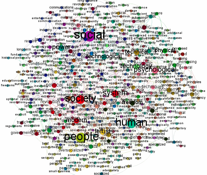
The one I have chosen has previously been analyzed by Seth Long (Text Network and Corpus Analysis of the Unabomber Manifesto). The Unabomber Manifesto is a 35,000 word document from 1995 entitled "Industrial Society and its Future", written by Theodore (Ted) Kaczynski, which is basically a critique of contemporary techno-capitalist society. A textual analysis is of interest because, as Seth notes: "The motives of all authors — or at least their traces — are always left behind in the lexical choices of their texts. Deliberate, written language is like a rhetorical fingerprint."

Textual analyses

Seth Long's textual analysis procedure was:

1. import the text into an analytical tool (in this case AutoMap) in order to remove trivial words (eg. articles, conjunctions, pronouns), and to reduce inflected words to their base form;
2. use the same tool to quantify what words are connected to what other words and how often (in this case using a two-word gap);
3. import the result into a a network analysis tool (in this case Gephi) in order to visualize the semantic connections; each word is visualized as a node in the network, and words that appear next to each other appear as edges in the network.

According to Seth:

The two most important network visualizations, in my opinion, show nodes with the highest levels of Betweenness Centrality and the highest levels of Degree Centrality. The latter measures how many total connections a node has to other individual nodes. The former measures whether or not a node is connected to other nodes that themselves have many connections. 

In a textual network, a word with high degree centrality is a word used in connection with a myriad of other words. This simply tells you that a word is used frequently in a text and in a variety of contexts. A word with high betweenness centrality is a word used frequently and in conjunction with other words that also connect to other nodes to form community clusters. This tells you that a word is not only used frequently and not only in many contexts but also that it is used in connection with words that also do a lot of semantic work in the text. A word with high betweenness centrality is a word through which many meanings in a text circulate.

Nodes with the greatest Degree Centrality in the text

Nodes with the greatest Betweenness Centrality in the text

The size of the words in the two networks represents their "amount" of centrality (ie. their importance). Clearly, these networks are very complex, and it would be best to simplify them. Seth does this in some of his other textual analyses, where he uses "one of Gephi’s degree range tools to hide the most disconnected nodes, thereby ‘cleaning’ the visualization of all but the most prominent clusters and connections" (eg. see Meaning circulation in Lolita). This has not been done in this example.

I will not provide an interpretation of these two networks, which you can find in Seth's original post. The basic conclusion is that "Kaczynski is a primitivist who loves nature more than humanity."

Seth also notes:

One thing a text network does, beyond providing an interesting visualization, is to point the researcher in the direction of terms and n-grams that might be explored more granularly in a corpus analysis tool, such as the NLTK [Natural Language Toolkit]. It provides a map of a text’s semantic circulation, a map that can be followed when we return to the world of pure textuality.

The two corpus analyses that Seth Long provides are a histogram of the most frequent words, and a graph of where in the text the most frequent words fall (beginning, middle, end, throughout, etc).

Phylogenetic analyses

We can now compare these analyses to the use of phylogenetic trees and networks as heuristic tools for data analysis and display. The objective is the same as for the above analyses, and the general approach is also very similar. The main difference, as explained above, is that the nodes and edges are inferred rather than observed. This means that the words appear only at the ends of terminal edges, rather than being scattered throughout the network.

These analyses involve:

1. remove trivial words, count the frequency of the remaining words, simplify the network by choosing how many of the words to display (50 in this case), and record their location in the text;
2. calculate the semantic "distance" between words based on their co-occurrence in a sliding window (in this case 20 words), using some similarity measure (in this case the jaccard coefficient); 
3. visualize the distances as an unrooted phylogenetic tree, in this case a neighbor-joining tree calculated using TreeCloud;
4. visualize the distances as an unrooted phylogenetic network, in this case a neighbor-net (a splits graph) calculated using SplitsNetworkCloud.

TreeCloud of the text

NetworkCloud of the text

In these phylogenetic analyses, the size of the words represents their frequency in the text, and the colour of the words represents their location in the text (red near the beginning, blue near the end). This adds the corpus analyses to the network visualization, making the graphs more informative. This can happen because the visualization itself is the inferred network, rather than the visualization summarizing various aspects of centrality of the underlying observed network.

The relative distance between two words in the text is given by the relative length of the path between them in the tree or network. Note that the "clean-up" of the graphs, by restricting the number of included words, helps a lot with the interpretation (as it would if also applied to the previous two graphs).

The phylogenetic tree focuses on certain of the word connections, rather than trying to display them all — it tries to infer which connections are "important" based on the measure of semantic distance, rather then connecting all nearby words. The interpretations from the tree are similar to those from the previous networks, but in many ways the interpretations are displayed more directly by the inferred (phylogenetic) graph than by summarizing centrality (either degree or betweenness).

Finally, the network is much more complex than the tree, which is often the case. Note that for the tree the edge lengths are all equal, but in the network the "average" distance between two words is given by the length of the path between them. This is just for illustrative purposes, as the tree could be drawn with variable edge lengths or the network drawn with unit edge lengths. The main reason for using unit edge lengths is that the terminal edges are often very long and the structure of the tree or network is hidden in the centre, as discussed by Gambette et al. (2012).

The main patterns that the network adds to the tree are: (a) "human" is separately associated with "control" and "behavior" on one hand and "beings" on the other; (b) "power" is separately associated with "process" and "autonomy" on one hand and "satisfy" on the other; and (c) "primitive" is separately associated with "individuals", "societies" and "groups" on one hand and "modern" and "man" on the other.

Conclusion

The phylogenetic approach is helpful because it focuses on certain of the network connections, rather than trying to display them all, as do the other networks. It cannot separately analyze concepts like degree and betweenness, and so information is lost; but this is traded off against the ability to include corpus analyses such as word frequency and location. Phylogenetic trees and networks can thus be valuable tools for textual analysis.

The TreeCloud was introduced by Gambette and Véronis (2010).  If you read French, then examples are presented by Amstutz and Gambette (2010) and by Gambette and Martinez (2012) (the latter has a comparison with some other multivariate data anlayses).

Thanks to Philippe Gambette for producing the NetworkCloud.

References

Amstutz D., Gambette P. (2010) Utilisation de la visualisation en nuage arboré pour l'analyse littéraire. JADT'10: 10th International Conference on Statistical Analysis of Textual Data.

Gambette P., Gala N., Nasr A. (2012) Longueur de branches et arbres de mots. Corpus 11: 129-146.

Gambette P., Martinez W. (2012) L'affaire du Mediator au prisme de la textométrie. Manuscript.

Gambette P., Véronis J. (2010) Visualising a text with a tree cloud. In: Locarek-Junge H., Weihs C. (eds) Classification as a Tool of Research, Proceedings of IFCS'09 (11th Conference of the International Federation of Classification Societies), pp. 561-570.

Distortions and artifacts in Principal Components Analysis for analysis of genome data

It is perfectly clear from examples in the genomics literature that there is a problem occurring with the use of Principal Components Analysis (PCA) ordinations, and that it is apparently going undetected by users. This problem involves a spurious second axis in the output graph that is a curvilinear function of the first axis. The danger is that the ordination diagrams will be interpreted as showing biological patterns (see François et al. 2010; Arenas et al. 2013), when these patterns are not in the original datasets. I illustrate this problem here using some very simple datasets, and point to some examples of it in the literature. I then suggest some possible solutions, including the use of phylogenetic networks.

Introduction

Genomic data are multivariate, in the sense that we have multiple characters (the nucleotide sequences) for multiple organisms. "Ordination" is the term used when we arrange the multivariate data in a rational order, which is then usually displayed as a scatter plot, with the points representing the organisms. The spatial relationships of the points on the graph then indicate how similar the organisms are to each other (based on their genomes) — close points are more similar to each other than are distant points, as shown by the example in the first figure.

Salmela et al. (2011), Figure 2d.
Each dot represents the genome of one Swedish person,
coloured according to their geographical location within northern Sweden.

There are many mathematical techniques for ordination, although they fall into two main groups: (i) eigenanalysis methods, and (ii) non-metric multidimensional scaling methods. These methods have a long history in some parts of biology, for example in ecology (Gauch 1982; Jongman et al. 1987; Kent & Coker 1992; Leps & Smilauer; Legendre & Legendre 2012), although they are virtually unknown in other parts. (Note: the eigenanalysis ordinations are sometimes confusingly called metric multidimensional scaling ordinations.)

The eigenanalysis method called Principal Components Analysis (PCA) was introduced by Patterson et al. (2006) to the study of genomic data, having previously been introduced into genetics by Menozzi et al. (1978)Cavalli-Sforza and Edwards (1964), and it has become quite popular in the literature since then. The basic idea is to summarize the data by calculating the correlation coefficient between each pair of organisms, and then to display as much as possible of the common pattern of variation along the first ordered axis of the graph, and as much of the remainder along the second axis, and so on. The different axes are expected to show independent patterns of genetic relationship among the organisms, with the first axis showing the most important pattern, the second axis the second-most important pattern, and so on.

However, ecologists have long known that the first two components of a PCA (and related eigenanalysis techniques such as correspondence analysis) often show an arching pattern, which is a mathematical artifact of the eigenanalysis rather than a real biological pattern in the original data (Gauch et al. 1977). This is most apparent when the sampling units cover a long ecological gradient and those samples at each end of the gradient have few species in common (Minchin 1987; see also this blog post). This is called the Arch Effect (or the Horseshoe Effect, or the Guttman Effect), in which the second axis is curved and twisted relative to the first axis, and thus the axes are not independent of each other.

The problem illustrated

Basically, the distortion involves the data pattern being displayed using one more axis than is needed for that data pattern. That is, a 1-dimensional pattern is displayed using 2 dimensions, instead, and a 2-dimensional pattern is displayed using 3 dimensions, etc. I will first illustrate this with a simple 1-dimensional pattern.

This first dataset consists of 20 nucleotide sequences. Each sequence consists of only two nucleotides (19 A and 5 C), and the pattern of Cs forms a simple gradient (ie. there is only one pattern in the data). This gradient can be displayed using only one ordination axis, which would arrange the taxa in order from Taxon_1 to Taxon_20. However, note that the patterns at the two ends of the gradient have nothing in common as far as the pattern of Cs is concerned.

The gradient dataset.

The next figure is the Principal Components Analysis (PCA) ordination diagram of these data. Note that the 1-dimensional pattern is displayed using 2 dimensions, arranging the 20 taxa in an arch rather than in a straight line. (Note that the open part of the arch can face either up or down; in this case it happens to face up.) So, it appears in the scatter plot that Taxon_1 and Taxon_20 are rather similar to each other (ie. they are near each other), which is not true. Furthermore, the dots are not equally spaced, which they should be given the pattern in the original data. The second dimension, along with the unequal spacing of the points, is a mathematical artifact of the eignenanalysis rather than a pattern in the data. It is caused by the unimodal distribution of the pattern of Cs along the gradient.

PCA ordination of the gradient data.
Not all of the taxa are labelled.

The second dataset consists of 24 nucleotide sequences. Each sequence consists of three nucleotides (8 A, 5 C and 4 T), and the pattern of Cs forms one gradient while the pattern of Ts forms a second gradient (orthogonal to the first one). These two independent patterns can be displayed using two ordination axes, which would arrange the taxa in a 6x4 rectangular grid. (If this is not clear, look at the bottom two figures of this post.)

The grid dataset.

This next figure is the PCA ordination diagram of these data. Note that the 2-dimensional pattern is displayed using 3 dimensions, only two of which are actually shown in the diagram. (It is standard to show only the first two axes, on the assumption that these contain most of the important information.) These axes arrange the 24 taxa in an arch in the first two dimensions, rather than in a straight line, and then separate pairs of taxa along the third axis. So, in two dimensions pairs of taxa appear to sit on top of one another, indicating a similarity that is not present in the original dataset. Once again, the use of the third dimension is an artifact of the eignenanalysis rather than a pattern in the data. It is caused by the unimodal distribution of the patterns of Cs and Ts along the two gradients.

PCA ordination of the grid data.

Clearly, when the samples form gradients then eigenanalysis is not an appropriate ordination technique, although it is very useful under many other circumstances. This problem with gradients has previously been pointed out for genomic data when they form a clinal geographical pattern (Novembre & Stephens 2008; Reich et al. 2008), but clearly the problem involves much more than just geographical patterns. Also, the problem is being ignored by users — most of the examples below were published after the paper by Novembre & Stephens.

Literature examples

The Arch Effect has appeared repeatedly in the genomics literature (often produced using the SmartPCA, Plink or Eigenstrat computer programs), and some examples are illustrated here. Note that the axes are not always in the same orientation, but the arch should be found on axis 2 relative to axis 1, and it can be oriented either up or down.

These first two examples come from the very paper that first introduced PCA to genomics studies.

Patterson et al. (2006), Figure 5.

Patterson et al. (2006), Figure 8.

These next two examples are from studies of genomic data from Scandinavia.

Salmela et al. (2011), Figure 2c.

Skoglund et al. (2012), Figure 1c.
Note that axis 1 is shown vertically.

The next two examples also come from worldwide genome studies. Note that the second of these refers to the ordination as metric multidimensional scaling (MDS).

Stoneking & Krause (2011), Box 1a.

Jakobsson et al. (2008), Figure 1d.

The next two examples also come from a worldwide genome study, but in this case the relationship of the Arch Effect to the geographical sampling is made explicit.

Wang et al. (2012), Figure 1b.

Wang et al. (2012), Figure 5b.

The next example illustrates rotation of the ordination axes, so that the arch is now aligned along the two axes.

Novembre and Ramachandran (2011), Figure 4e.

Finally, the Gene Expression blog has an example, where the ordination is called a metric multidimensional scaling (MDS) ordination. This is based on ~3,000 individuals and 250,000 SNPs.

Possible solutions

There are three possible solutions to the Arch Effect problem in eigenanalysis ordinations.

First, one can try to mathematically correct the distortion. This approach was actively pursued in ecology via what is known as detrending and rescaling (Hill & Gauch 1980), in which the axes are forced to be independent of each other after the eigenanalysis. This approach works, in the sense that the Arch Effect disappears, but it has the drawback that all relationships between the axes are removed, including those that require more than one dimension to be displayed (Palmer 1993). So, while this method is still commonly encountered in the ecological literature, it is not uniformly recommended.

This approach is illustrated in the next figure, which is a Detrended Correspondence Analysis (DCA, with detrending by second-order polynomials) ordination analysis of the second of my simple datasets above. Note that the original 2-dimensional grid arrangement of the taxa is perfectly preserved, so that the ordination diagram is exactly as expected.

DCA ordination of the grid data.

The second, and most obvious, solution to the problem is not to use an eigenanalysis ordination in the first place. That is, not all ordination techniques produce the same result. In this case we could use a Non-metric Multidimensional Scaling (NMDS) ordination, instead. The latter is a very different type of technique, mathematically, which explicitly tries to arrange the points in the ordination plot so that their relative distances reflect as closely as possible the pairwise "distances" in the original dataset (here, a distance is the inverse of a similarity). This technique is known to avoid the Arch Effect (Minchin 1987).

This is illustrated in the next figure, which is a NMDS ordination analysis of the second dataset. Note that the original 2-dimensional grid arrangement of the taxa is almost perfectly preserved. The main disadvantages of NMDS are the computational time required, the difficulty of finding the optimal solution for large datasets (eigenanalysis is significantly faster; Zheng et al. 2012), and the fact that the number of ordination axes needs to be specified beforehand.

NMDS ordination of the grid data.
Not all of the taxa are labelled.

The third solution to the problem is to use a phylogenetic network to display the multidimensional data, rather than using an ordination. Conceptually, this is similar to the NMDS type of ordination, but it uses a line graph to display the results rather than using a scatter plot. I have illustrated this in the next blog post (Networks can outperform PCA ordinations in phylogenetic analysis), where I report that this solution works quite well, too.

Conclusion

Every time you see an arch in a PCA plot, you might very well be looking at a mathematical artifact. You should bear this in mind when you interpret the ordination pattern, especially if you wish to draw biological conclusions from the diagram. You will, of course, see plenty of PCA ordinations without any evidence of an arch, and these are probably safe to interpret naively.

PCA can be useful when we expect genomes to be monotonically related to one another, but this is likely to be rather rare in nature. It is much more likely that genomes will have nonlinear relationships, such as unimodal patterns, with a peak at an intermediate part of any gradients that are present. Under these circumstances it produces artifacts, which may be mistakenly interpreted as representing real biological patterns. Under these circumstances, an alternative method of multivariate analysis should be used.

More information about ordination techniques can be found at the Ordination Methods web page.

Note: updated Friday December 21 2012.

References

Arenas M, François O, Currat M, Ray N, Excoffier L (2013) Influence of admixture and paleolithic range contractions on current European diversity gradients. Molecular Biology and Evolution 30: 57-61.

Cavalli-Sforza L, Edwards AWF (1964) Analysis of human evolution. Proceedings of the 11th International Congress of Genetics, The Hague, 1963. Genetics Today 3: 923-933.

François O, Currat M, Ray N, Han E, Excoffier L, Novembre J (2010) Principal component analysis under population genetic models of range expansion and admixture. Molecular Biology and Evolution 27: 1257-1268.

Hill MO, Gauch HG (1980) Detrended Correspondence Analysis: an improved ordination technique. Vegetatio 42: 47-58.

Gauch HG (1982) Multivariate Analysis in Community Structure. Cambridge University Press, Cambridge.

Gauch HG, Whittaker RH, Wentworth TR (1977) A comparative study of reciprocal averaging and other ordination techniques. Journal of Ecology 65: 157-174.

Jongman RHG, ter Braak CJF, van Tongeren OFR (1987) Data Analysis in Community and Landscape Ecology. Pudoc, Wageningen.

Kent M, Coker P (1992) Vegetation Description and Analysis: a Practical Approach. Belhaven Press, London.

Legendre P, Legendre L (2012) Numerical Ecology, 3rd edition. Elsevier, Amsterdam.

Leps J, Smilauer P (2003) Multivariate Analysis of Ecological Data using Canoco. Cambridge University Press, Cambridge.

Menozzi P, Piazza A, Cavalli-Sforza L (1978) Synthetic maps of human gene frequencies in Europeans. Science 201: 786-792.

Minchin PR (1987) An evaluation of relative robustness of techniques for ecological ordinations. Vegetatio 69: 89-107.

Novembre J, Ramachandran S (2011) Perspectives on human population structure at the cusp of the sequencing era. Annual Review of Genomics and Human Genetics 12: 245-74.

Novembre J, Stephens M (2008) Interpreting principal component analyses of spatial population genetic variation. Nature Genetics 40: 646-649.

Palmer MW (1993) Putting things in even better order: the advantages of Canonical Correspondence Analysis. Ecology 74: 2215-2230.

Patterson N, Price AL, Reich D (2006) Population structure and eigenanalysis. PLoS Genetics 2: e190.

Reich D, Price AL, Patterson N (2008) Principal component analysis of genetic data. Nature Genetics 40: 491-492.

Salmela E, Lappalainen T, Liu J, Sistonen P, Andersen PM, Schreiber S, Savontaus ML, Czene K, Lahermo P, Hall P, Kere J (2011) Swedish population substructure revealed by genome-wide single nucleotide polymorphism data. PLoS One 6: e16747.

Skoglund P, Malmström H, Raghavan M, Storå J, Hall P, Willerslev E, Gilbert MT, Götherström A, Jakobsson M (2012) Origins and genetic legacy of Neolithic farmers and hunter-gatherers in Europe. Science 336: 466-469.

Stoneking M, Krause J (2011) Learning about human population history from ancient and modern genomes. Nature Reviews Genetics 12: 603-614.

Wang C, Zöllner S, Rosenberg NA (2012) A quantitative comparison of the similarity between genes and geography in worldwide human populations. PLoS Genetics 8: e1002886.

Zheng X, Levine D, Shen J, Gogarten SM, Laurie C, Weir BS (2012) A high-performance computing toolset for relatedness and Principal Component Analysis of SNP data. Bioinformatics 28: 3326-3328.