
This is a joint post by Timothy Holt and Guido Grimm
One ‘a-phylogenetic’ application of phylogenetic methods is the classification of stellar (in the widest sense) objects, so-called "astrocladistics" (see Didier Fraix-Burnet’s dedicated blog: astrocladistics.org). Traditionally, the objects would be characterized and their (dis)similarity translated into a plot (eg. using PCoA) or a tree (eg. a UPGMA tree). Such cluster analysis frameworks would then be the basis for the classification of the objects.
In ‘astrocladistics’, phylogenetic trees that fulfill the maximum parsimony or minimum evolution criteria, are used instead. But why should we stop with trees (see the prior blog post Astrocladistics: a network analysis)? For this post, we have used the matrices of a recent astrocladistic paper by Holt et al. (2018) to highlight an as yet under-explored application of phylogenetic methods in classification: exploratory data analysis (EDA).
Why exploratory data analysis
As noted in the earlier post on astrocladistics, one problem is that one infers phylogenetic trees based on a data sets that are not the product of an evolutionary process. Some objects may evolve from others (eg. a satellite may evolve from planetary ring matter), but this is not a dichotomous splitting process through time. And any non-dichotomous process can lead to tree-incompatible signals, which will then hamper tree inference in a biological context. Any tree using astral objects (galaxies, stars, planets, moons) as OTUs is per se a faux phylogeny (some examples for faux phylogenies are collected here and here).
Another problem is a data-inherent bias. The matrices are coded in a fashion that reflects an a priori hypothesis of derivation. For instance, by inferring that objects farther away are older and closer ones are younger, we can make hypotheses about maturation of galaxies, and hard-code this hypothesis into the data matrix. This will infer a tree that was coded into the matrix.
Guido’s starting argument is that when our main goal is classification and not inferring evolutionary relationships, the topology of the tree (or alternative trees) is the least of our concerns. What we want to know is to what degree our data converges to the same groupings, supports coherent classes. This is exploratory data analysis, and Neighbor-nets are then a powerful tool to visualize any differentiation pattern (see some recent a-biological examples: U.S. gun legislation, cryptocurrencies, where to retire Worldwide and within the USA)
Instead of inferring trees, as in the original paper about two satellite systems (Jupiter and Saturn), here we use the matrices to infer Neighbor-nets, map character support (non-parametric bootstrap support) on the resultant networks, and discuss the prospects and perils of ‘astro-Neighbor-nets’ when it comes to classification of astronomical bodies.
Data properties and analysis set-up
In order to construct the matrices, three different types of characteristics were used: dynamical, physical and compositional. Dynamical characteristics are the positions of the various satellites, how far they are away from the planet (semi-major axis), their inclination to the plane and eccentricity of their orbit. Several of the satellites also orbit opposite to the planet's rotation (they are on a retrograde orbit), which is also code. Physical characteristics are two properties of the satellites: their albedo, or how reflective they are, and their density. Any characteristics related to mass and size are specifically avoided, as this would hide any parent/daughter relationships resulting from breakups. The compositional characteristics are the most numerous ones in the analysis. These are binary characteristics indicating the presence/absence of chemical species, eg. water, iron, methane, etc.
Five of the characteristics, semi-major axis, inclination, eccentricity, albedo and density, are ordered and continuous. These prose a problem for standard cladistic analysis using parsimony, which needs discrete character states. Hence, these characteristics are binned using a python program. Each character-set is binned independently, and for each of the Jovian and Saturnian systems. The aforementioned python program iterates the number of bins until a linear regression model between binned and unbinned sets achieves a coefficient of determination (r2) score of > 0.99. All characteristics are binned in a linear fashion, with the majority increasing in progression. The exception to the linear increase is the density character set, with a reversed profile. All of the continuous, binned characteristic sets are (by definition) ordered characters.
Thus, the matrices comprised two sorts of characters with strongly different properties, when it comes to explicit inferences: binary characters, and highly ordered characters (the binned ones) with up to 11 states. For the graphs used here, we didn’t apply any weighting, which means that in the most extreme case complete difference in a binned character counts 11-times more than a difference in any of the binary characters. This bias is compensated to some degree by the number of binary characters (33, with 31 variable) vs. binned characters (5), when restricting the analysis to well-known planetary objects.
The matrices are comprehensive, and include little-known objects with a lot of missing data (>80% of the characters cannot be scored), which should be included. A matrix-based classification makes most sense, when one uses character sets that are defined for most or all of the objects. Thus, to see how the little-known objects relate to the well-known, we eliminated all poorly covered characters, leaving us with two binary and five binned ones. To not lose the information from the binary characters when calculating the inter-object distances, we gave them a weight of 7–8. This ensures that a 0↔1 difference in a binary character more or less equals the maximum possible difference in a binned character (on average 8 bins for the Jupiter dataset, and7 for the Saturn data set).
 |
| Fig. 1 The orbits of the satellites in the Jovian satellite system. Colours represent traditionally recognized groups. |
The Jovian moons (and ring)
The Jovian system (Fig. 1) is dominated by the famous Galilean satellites (moons): Io, Europa, Ganymede, and Callisto. In between these moons and Jupiter there is a faint ring system, and four small satellites, the Amalthea family. Outside the Galilean system, there is a system of 67 small irregular satellites that have much wilder orbits, some going in the opposite direction to the other satellites. These are thought to be captured asteroids.
As seen in Fig. 2, the data analysis supports a somewhat tree-like network. The Galilean Group (the large moons), the association of Amalthea with Jupiter’s Main Ring, and the Himalia Family, but it rejects the traditional division of the remaining well-known moons (captured asteroids) into three families: two of the three Pasiphae Family satellites are very similar to Carme. Although Ananke is somewhat different, it is substantially more similar to Carme and the Pasiphae Family satellites than the inter-group differentiation found elsewhere. One commonly shared idea about classification is that one should erect classes that have similar quality and are defined by high intra-class coherence and inter-class differentiation.
 |
| Fig. 2 Neighbor-net of Jovian moons, well-covered by data (<1% or no missing data). Colouration addresses traditionally recognised groups, same colours used as in Fig. 1. |
By reducing the character set to those characters that are defined for most or all moons, we naturally take away some of the potential differentiation. Nonetheless, the resulting graph (Fig. 3) provides a structure that may well be used to place less-known objects, identify their closest best-known counterpart(s), erect a classification, and discuss current classification schemes.
 |
| Fig. 3 Neighbor-net of all Jovian moons based on a distance-matrix reflecting the known (scored) similarity and differences. Colouration as above. |
We can see that we lose differentiation within the well-known (and well-supported; Fig. 2) groups, especially regarding the distinctness between members of the Galilean Group and to the Amaltheae Family. However, the basic structure of the graph remains the same. Based on the scored data, the Ananke, Pasiphae and Carmes Families are not supported. A sub-division may be possible, but would require some re-shuffling of the moons. For instance, a group including Ananke-like satellites would not include Euporie, Iocaste and Hermippe, but may include Callirhoe. A Pasiphae s.str. group would make sense when excluding Aoede, Helike, Sinope, Autonoe, and Eurydome, with the latter three being (nearly) identical to Carmes or members of the Carmes Family.
 |
| Fig. 4 The orbits of the satellites in the Saturnian satellite system. Colours represent traditionally recognised groups. |
The Saturnian moons and rings
The Saturn system (Fig. 4) is similar to of the Jupiter one.
The ring structure is one of Saturn’s most distinctive features, with structures seen even with a modest telescope. Imbedded in the rings are small moon-lets. The co-orbitals Janus and Epimetheus, just outside the main rings, swap orbits every four years. There are eight mid-sized satellites, including Titan, a small world in itself with a methane-based weather system. Of the other icy satellites, Mimas, Enceladus, Tethys, Dione and Rhea, are embedded in the diffuse E-ring. The source of this ring is cryovolcanic plumes on Enceladus, a possible location for life beyond Earth.
Unique to the Saturn system are Trojan satellites, in the same orbit as their parent satellites, one 60o ahead, and 60o behind. Tethys has Telesto and Calypso as Trojan satellites, while Helene and Polydeuces are Trojan satellites of Dione. Between the orbits of Mimas and Enceladus, there are the Alkyonides (Methone, Anthe and Pallene) recently discovered by the Cassini spacecraft. Each of the Alkyonides have their own faint ring arcs comprised of similar material to the satellite.
As with Jupiter, there is also a system of 38 small irregular satellites outside the inner system. This system is dominated by Phoebe — at ~240 km across it is six times the size of the next largest irregular. It is also the only irregular satellite to have its photo taken, with the Cassini spacecraft flying within 2,000 km of the surface, taking high-res images as it went. Using these new data, a picture is emerging of Phoebe as a captured outer solar system object.
For Jupiter’s smaller sibling (Saturn), a less tree-like network is inferred (Fig. 5). Since it is not the product of an evolutionary process in a biological sense (ie. a phylogeny), but instead including patterns related to parent/descendant relationships (rings-moons, breakups), we should not necessarily expect tree-like graphs.
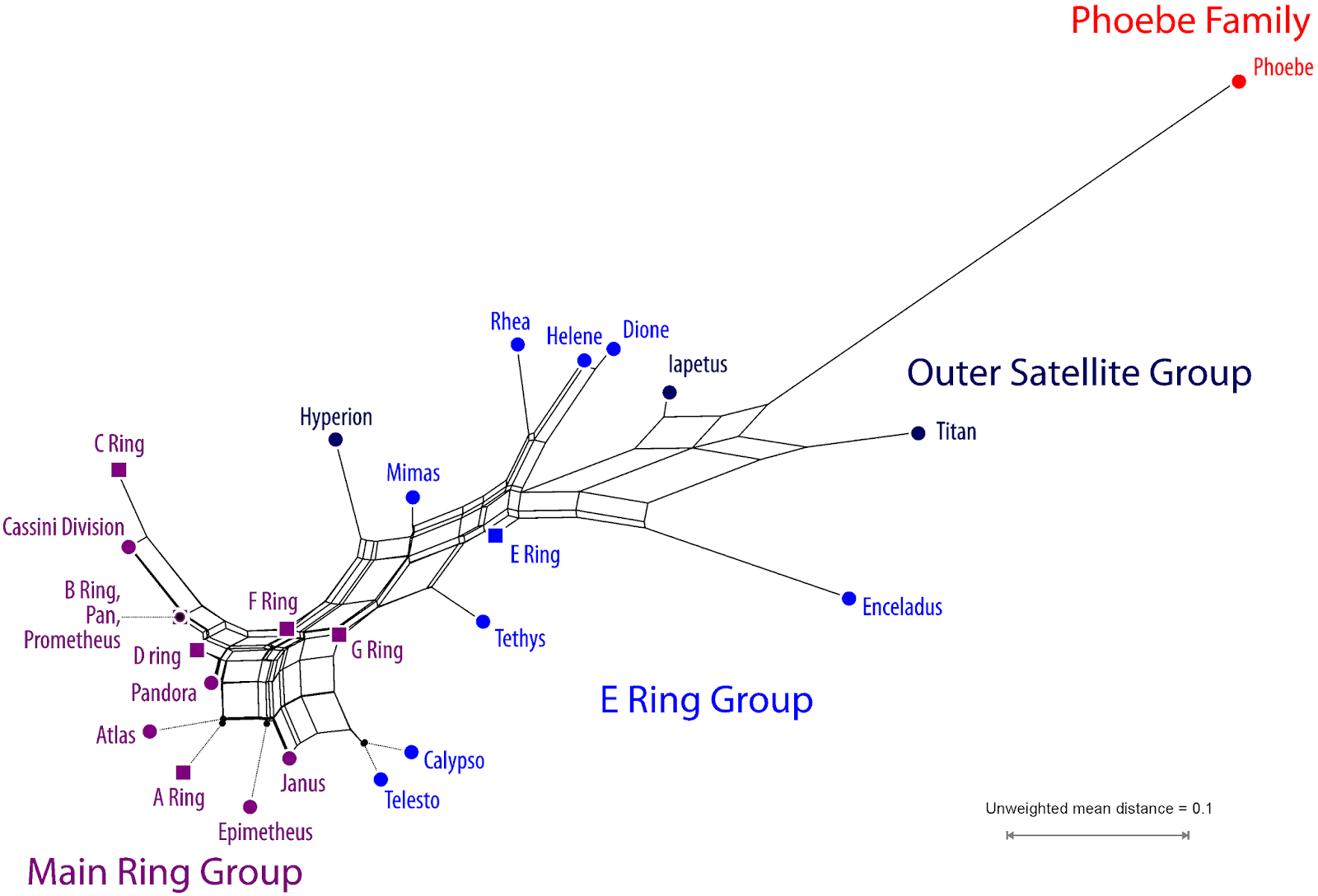 |
| Fig. 5 Neighbor-net of well-known Saturnian planetary objects (<1% or no missing data). Colouration addresses traditionally recognised groups using the same colours than in Fig. 4. |
Nonetheless, the graph could be the basis of an objective classification. The elements of the ‘Main Ring Group’ have high intra-group coherence, but also include Calypso and Telesto of the ‘E Ring Group’. On the other hand, the ‘Outer Satellite Group’ is very heterogeneous. One straightforward option would be to fuse this group with the E Ring Group; another is to exchange Enceladus for Hyperion. The Norse Group’s (= Phoebe Family) representative Phoebe is clearly distinct from any other object and would need a class of its own.
As in the case of Jupiter ,we can add and try to classify the remaining little-known objects (Fig. 6), to some degree.
 |
| Fig. 6 Neighbor-net of all Saturnian moons and rings based on a distance-matrix reflecting the known (scored) similarity and differences. Colouration as above. |
In contrast to Jupiter, the reduced character set (just four characters, one binary, three binned-ordered) loses the differentiation between objects of the Main Ring, E Ring and Outer Satellite groups included in Fig. 5. They are virtually identically for these characters. The two groups not covered in Fig. 5, the Siarnaq (named after Inuit gods) and Albiorix Family (Gallic gods), are close to each other. The Albiorix Family forms a distinct subset of the Siarnaq Family. The moons of the coherent Phoebe Family (named after Norse mythological figures) are all close to each other, and this group includes various newly discovered satellites. Interesting is also the position of the Phoebe Ring compared to its name-giving moon and the remainder of the Phoebe Family.
Comparison with the tree-based analyses
In comparison with the astrocladistical work of Holt et al. (2018), the network-based analysis captures most of the meta-structure of the satellite classifications.
Compared with the Jovian trees, the network-based analysis shows the distinction between the inner Galilean group and the outer ‘irregular’ satellites and separates the Himalia family. The differences are in how each of the analyses handles the retrograde irregulars, the Pasiphae, Carme and Ananke families. It should be noted that these bodies are woefully under-studied, and have very little information available, making any inferences difficult.
In Holt et al.’s trees, the Ananke, Carme and Sinope subfamiles are unresolved, but are supported using Multivariate Hierarchical Cluster Analysis (example provided in Fig. 7). This method uses clustering in parameter space to justify collisional families. Though the particular members are different, the network-based analysis still identifies clusters around the largest irregular satellites, Anake, Sinope, Carme and Pasiphae. This further supports further the theory that these families are remnants of collision breakups. As usual with science, there is far more work to be done here.
 |
| Fig 7: Clustering of several Jovian Irregular satellites in three dimensional parameter space using Semi-major axis (a), eccentricity (e) and inclination (i). |
In the Saturnian system, the outer satellites also prove to be problematic. Holt et at. split the Aegir and Ymir subfamilies from within the Phoebe family. These subfamilies are distinct from Phoebe and its ring, following a narrative of a different origin for Phoebe and the rest of the irregular satellites. The capture of Phoebe would have major disruptive effects on the satellites. As the dynamical characteristics play such a large role, they are the only information available for some of the satellites, so that little sub-structuring can be seen. As with the Jovian irregular satellites, more information is needed.
The inner system of Saturn also warrants mention, particularly the case of Telesto and Calypso, the Trojans of Tethys. In the network analysis, they are associated with main ring objects, rather than with Tethys itself. There is a possibility that these two Trojans are captured main-ring objects, and this would support that hypothesis. Dione, and its Trojan Helene, are both closely associated with one another in both analyses, indicating a parent/daughter relationship (keep in mind that phylogenetic trees cannot discern between parent/daughter and sister relationships).
 |
| Phoebe as seen by the Cassini spacecraft, NASA/JPL/Space Science Institute, PIA06064 (the NASA provides more than 1000 media files covering the Cassini-Huygens mission) |
Boldly gone – networks as tools in classification
The idea discussed here appears worth exploring — using distance-based or other (meta-)phylogenetic networks for the classification of objects not necessarily following any phylogeny. It has some obvious advantages over astrocladistics (especially when using maximum parsimony as the tree-optimizing criterion) or traditional classification methods (PCoA, simple clustering approaches):
- Distance-matrices are easy and quick to generate based on any data; and they can also be used for more traditional classification means such as PCoA.
- Neighbor-nets are very quick to calculate, and can capture more aspects of the actual differentiation than can cluster analysis (e.g. UPGMA trees, PCoA) or astrocladistic methods; in some sense they represent a fusion of the best aspects of both approaches.
- In contrast to a tree, where tree-incompatible signals can massively distort branch-length patterns, or rogue objects interfere with establishing a finely resolved topology, a Neighbor-net can be straightforwardly interpreted regarding group coherence.
However, using the Neighbor-net as a basis for classification, groups also allows us to quickly test for character sampling bias, eg. by re-calculating the distance input matrix using weighting schemes, or different distance calculations (eg. instead of binning the continuous characters, they could be used as-is), or reduced character or taxon sets. Also, when it comes to classifying non-living objects, it’s always good to keep it as simple as possible, while being able to explore the signal in the data matrix.
More results, the data matrices used, and the template analysis files can be found on figshare. The archive includes also the (simple) NEXUS-formatted files with the PAUP* command blocks we used for the analyses. The one for Jupiter is fully annotated with comments on the code lines for PAUP* to assist inexperienced users and to facilitate export (and subsequent) import into SplitsTree.
The archive includes also the code for and results of a full bootstrap-support analysis (currently two optimality criteria: Least-squares and Maximum parsimony, Maximum likelihood to be added) — even when preferring the astrocladistic approach, networks are handy to summarize the bootstrap pseudoreplicate sample.
Reference
Holt TR, Brown AJ, Nesvorný D, Horner J, Carter B (2018) Cladistical analysis of the Jovian and Saturnian satellite systems. Astrophysical Journal 859(2): 97, 20 pp; arXiv: 1706.0142
These are distance trees calculated with distance methods. They belong to phenetics, not to cladistics.
ReplyDeleteWe are talking about moons here, not biological evolution and concepts.
ReplyDeleteThe neighbour-nets here are not "astrocladistics", they are per se "phenetic" because of the data used. The same could be argued for any tree inferred on these data (parsimony-optimised or otherwise), but "astrocladistics" is the terminology used when classifying astromical objects using tree-inference.
Generally, I would caution against using biological-philosophical terminology ("phenetic", "phylogenetic", "cladistic") for anything not dealing with an organism.
PS A neighbour-joining tree (during the Phylogenetic Wars often deprecatorily addressed as "phenetic" because it relies on a cluster algorithm, like the algorithm to infer a neighbour-net) based on biological data fulfills either the minimum evolution or least-squares optimality criteria. The cluster algorithm is just a short-cut to find the optimal tree. Thus, any NJ tree fulfilling one of these criteria is a phylogenetic tree (see e.g. Felsenstein, Inferring Phylogenies, 2004 (there is also a post by David on this blog, I think). Its clades could be used for a cladistic classification (not to be confused with phylogenetic classification following Hennig; see e.g. this post October last year)
Neighbour-nets are not necessarily phylogenetic networks (see also this post, but a sort of meta-phylogenetic network. If based on data from evolving organisms.