Cloudograms and data-display networks

I have previously noted that splits graphs are a logical way to present the results of Bayesian analyses (We should present bayesian phylogenetic analyses using networks). Bayesian analyses are concerned with estimating a whole probability distribution, rather than producing a single estimate of the maximum probability. Thus, the result of a Bayesian phylogenetic analysis should not be as a single tree (the so-called MAP tree or maximum a posteriori probability tree), but should instead show the probability distribution of all of the sampled trees. This can easily be done with a consensus network, as illustrated by example in the previous blog post.

An interesting alternative way of visualizing the probability distribution of trees is what has been called a Cloudogram, an idea introduced by Remco R. Bouckaert (2010, DensiTree: making sense of sets of phylogenetic trees. Bioinformatics 26: 1372-1373). This diagram superimposes the set of all trees arising from an analysis. Dark areas in such a diagram will be those parts where many of the trees agree on the topology, while lighter areas will indicate disagreement. This idea can be best illustrated by a few published examples.

The first cloudogram is from Figure 4 of Chaves JA, Smith TB (2011) Evolutionary patterns of diversification in the Andean hummingbird genus Adelomyia. Molecular Phylogenetics and Evolution 60: 207-218.

In this case the MAP tree has been superimposed on the cloudogram.

Species-tree with the highest posterior probability (PP > 80) superimposed upon
a cloudogram of the entire posterior distribution of species-trees recovered in BEAST.
Areas where the majority of trees agree in topology and branch length are shown as
darker areas (well-supported clades), while areas with little agreement as webs.

The next one is from Figure 2 of Pabijan M, Crottini A, Reckwell D, Irisarri I, Hauswaldt JS, Vences M (2012) A multigene species tree for Western Mediterranean painted frogs (Discoglossus). Molecular Phylogenetics and Evolution 64: 690-696.

Posterior density of 2700 species trees (‘‘cloudogram’’) representing the entire posterior distribution
of species trees (270,000 trees post-burnin) from the BEAST analysis based on seven nuclear loci and
4 mitochondrial gene fragments. The species tree with the highest posterior probability is nested within
the set; values indicate posterior probabilities associated with this consensus tree. Areas where many
species trees agree on topology and/or branch lengths are densely colored.

The next one is from Figure 1 of Lerner HR, Meyer M, James HF, Hofreiter M, Fleischer RC (2011) Multilocus resolution of phylogeny and timescale in the extant adaptive radiation of Hawaiian honeycreepers. Current Biology 21: 1838-1844.

In this case the data are more tree-like than the previous two examples.

Cloudogram showing all trees resulting from a Bayesian analysis of whole
mitogenomes (19,601 trees; 14,449 bps). Variation in timing of divergences is
shown as variation (i.e., fuzziness) along the x axis. Darker branches represent a
greater proportion of corresponding trees. All nodes have support values >0.99.

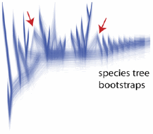
The final one is from  Figure 2 of McCormack JE, Faircloth BC, Crawford NG, Gowaty PA, Brumfield RT, Glenn TC (2012) Ultraconserved elements are novel phylogenomic markers that resolve placental mammal phylogeny when combined with species-tree analysis. Genome Research 22: 746-754.

This analysis involves bootstraps rather than Bayesian samples, showing that the same principle applies.

Evolutionary history of placental mammals resolved from conflicting
gene histories. Widespread consensus among 1000 species-tree bootstrap
replicates of the same 183-locus data set. STEAC trees are depicted because
the branch lengths allow for better visualization of branching patterns, but
STAR results supported the same topology. Cones emanating from terminal
tips of species trees (red arrows) indicate disagreement among bootstrap
replicates.

It would be nice to illustrate this further by direct comparison with a splits graph of the same dataset that I used in the previous blog post. Unfortunately, the computer program available (DensiTree) has the same practical limitation as the SplitsTree program (as mentioned in the previous post) — it does not read the MrBayes ".trprobs" file because it ignores the tree weights. This means that one has to enter the entire treefile (with thousands of trees), and I have not yet done that. Moreover, the program relies very much on having branch lengths for each tree — the output is really quite odd without them, with the taxa appearing in a series of steps rather than connected by straight branches. My previous analysis did not use branch lengths, as they are not needed for the consensus network, in which edge lengths represent support rather than character evolution.